If you're seeing this message, it means we're having trouble loading external resources on our website.
If you're behind a web filter, please make sure that the domains *.kastatic.org and *.kasandbox.org are unblocked.
To log in and use all the features of Khan Academy, please enable JavaScript in your browser.

Statistics and probability
Course: statistics and probability > unit 12, hypothesis testing and p-values.
- One-tailed and two-tailed tests
- Z-statistics vs. T-statistics
- Small sample hypothesis test
- Large sample proportion hypothesis testing
Want to join the conversation?
- Upvote Button navigates to signup page
- Downvote Button navigates to signup page
- Flag Button navigates to signup page

Video transcript

User Preferences
Content preview.
Arcu felis bibendum ut tristique et egestas quis:
- Ut enim ad minim veniam, quis nostrud exercitation ullamco laboris
- Duis aute irure dolor in reprehenderit in voluptate
- Excepteur sint occaecat cupidatat non proident
Keyboard Shortcuts
Lesson 3: probability distributions, overview section .
In this Lesson, we take the next step toward inference. In Lesson 2 , we introduced events and probability properties. In this Lesson, we will learn how to numerically quantify the outcomes into a random variable. Then we will use the random variable to create mathematical functions to find probabilities of the random variable.
One of the most important discrete random variables is the binomial distribution and the most important continuous random variable is the normal distribution. They will both be discussed in this lesson. We will also talk about how to compute the probabilities for these two variables.
- Distinguish between discrete and continuous random variables.
- Compute probabilities, cumulative probabilities, means and variances for discrete random variables.
- Identify binomial random variables and their characteristics.
- Calculate probabilities of binomial random variables.
- Describe the properties of the normal distribution.
- Find probabilities and percentiles of any normal distribution.
- Apply the Empirical rule.

- school Campus Bookshelves
- menu_book Bookshelves
- perm_media Learning Objects
- login Login
- how_to_reg Request Instructor Account
- hub Instructor Commons
Margin Size
- Download Page (PDF)
- Download Full Book (PDF)
- Periodic Table
- Physics Constants
- Scientific Calculator
- Reference & Cite
- Tools expand_more
- Readability
selected template will load here
This action is not available.
8.1.3: Distribution Needed for Hypothesis Testing
- Last updated
- Save as PDF
- Page ID 10975

\( \newcommand{\vecs}[1]{\overset { \scriptstyle \rightharpoonup} {\mathbf{#1}} } \)
\( \newcommand{\vecd}[1]{\overset{-\!-\!\rightharpoonup}{\vphantom{a}\smash {#1}}} \)
\( \newcommand{\id}{\mathrm{id}}\) \( \newcommand{\Span}{\mathrm{span}}\)
( \newcommand{\kernel}{\mathrm{null}\,}\) \( \newcommand{\range}{\mathrm{range}\,}\)
\( \newcommand{\RealPart}{\mathrm{Re}}\) \( \newcommand{\ImaginaryPart}{\mathrm{Im}}\)
\( \newcommand{\Argument}{\mathrm{Arg}}\) \( \newcommand{\norm}[1]{\| #1 \|}\)
\( \newcommand{\inner}[2]{\langle #1, #2 \rangle}\)
\( \newcommand{\Span}{\mathrm{span}}\)
\( \newcommand{\id}{\mathrm{id}}\)
\( \newcommand{\kernel}{\mathrm{null}\,}\)
\( \newcommand{\range}{\mathrm{range}\,}\)
\( \newcommand{\RealPart}{\mathrm{Re}}\)
\( \newcommand{\ImaginaryPart}{\mathrm{Im}}\)
\( \newcommand{\Argument}{\mathrm{Arg}}\)
\( \newcommand{\norm}[1]{\| #1 \|}\)
\( \newcommand{\Span}{\mathrm{span}}\) \( \newcommand{\AA}{\unicode[.8,0]{x212B}}\)
\( \newcommand{\vectorA}[1]{\vec{#1}} % arrow\)
\( \newcommand{\vectorAt}[1]{\vec{\text{#1}}} % arrow\)
\( \newcommand{\vectorB}[1]{\overset { \scriptstyle \rightharpoonup} {\mathbf{#1}} } \)
\( \newcommand{\vectorC}[1]{\textbf{#1}} \)
\( \newcommand{\vectorD}[1]{\overrightarrow{#1}} \)
\( \newcommand{\vectorDt}[1]{\overrightarrow{\text{#1}}} \)
\( \newcommand{\vectE}[1]{\overset{-\!-\!\rightharpoonup}{\vphantom{a}\smash{\mathbf {#1}}}} \)
Earlier in the course, we discussed sampling distributions. Particular distributions are associated with hypothesis testing. Perform tests of a population mean using a normal distribution or a Student's \(t\)-distribution. (Remember, use a Student's \(t\)-distribution when the population standard deviation is unknown and the distribution of the sample mean is approximately normal.) We perform tests of a population proportion using a normal distribution (usually \(n\) is large or the sample size is large).
If you are testing a single population mean, the distribution for the test is for means :
\[\bar{X} \sim N\left(\mu_{x}, \frac{\sigma_{x}}{\sqrt{n}}\right)\]
The population parameter is \(\mu\). The estimated value (point estimate) for \(\mu\) is \(\bar{x}\), the sample mean.
If you are testing a single population proportion, the distribution for the test is for proportions or percentages:
\[P' \sim N\left(p, \sqrt{\frac{p-q}{n}}\right)\]
The population parameter is \(p\). The estimated value (point estimate) for \(p\) is \(p′\). \(p' = \frac{x}{n}\) where \(x\) is the number of successes and n is the sample size.
Assumptions
When you perform a hypothesis test of a single population mean \(\mu\) using a Student's \(t\)-distribution (often called a \(t\)-test), there are fundamental assumptions that need to be met in order for the test to work properly. Your data should be a simple random sample that comes from a population that is approximately normally distributed. You use the sample standard deviation to approximate the population standard deviation. (Note that if the sample size is sufficiently large, a \(t\)-test will work even if the population is not approximately normally distributed).
When you perform a hypothesis test of a single population mean \(\mu\) using a normal distribution (often called a \(z\)-test), you take a simple random sample from the population. The population you are testing is normally distributed or your sample size is sufficiently large. You know the value of the population standard deviation which, in reality, is rarely known.
When you perform a hypothesis test of a single population proportion \(p\), you take a simple random sample from the population. You must meet the conditions for a binomial distribution which are: there are a certain number \(n\) of independent trials, the outcomes of any trial are success or failure, and each trial has the same probability of a success \(p\). The shape of the binomial distribution needs to be similar to the shape of the normal distribution. To ensure this, the quantities \(np\) and \(nq\) must both be greater than five \((np > 5\) and \(nq > 5)\). Then the binomial distribution of a sample (estimated) proportion can be approximated by the normal distribution with \(\mu = p\) and \(\sigma = \sqrt{\frac{pq}{n}}\). Remember that \(q = 1 – p\).
In order for a hypothesis test’s results to be generalized to a population, certain requirements must be satisfied.
When testing for a single population mean:
- A Student's \(t\)-test should be used if the data come from a simple, random sample and the population is approximately normally distributed, or the sample size is large, with an unknown standard deviation.
- The normal test will work if the data come from a simple, random sample and the population is approximately normally distributed, or the sample size is large, with a known standard deviation.
When testing a single population proportion use a normal test for a single population proportion if the data comes from a simple, random sample, fill the requirements for a binomial distribution, and the mean number of successes and the mean number of failures satisfy the conditions: \(np > 5\) and \(nq > 5\) where \(n\) is the sample size, \(p\) is the probability of a success, and \(q\) is the probability of a failure.
Formula Review
If there is no given preconceived \(\alpha\), then use \(\alpha = 0.05\).
Types of Hypothesis Tests
- Single population mean, known population variance (or standard deviation): Normal test .
- Single population mean, unknown population variance (or standard deviation): Student's \(t\)-test .
- Single population proportion: Normal test .
- For a single population mean , we may use a normal distribution with the following mean and standard deviation. Means: \(\mu = \mu_{\bar{x}}\) and \(\\sigma_{\bar{x}} = \frac{\sigma_{x}}{\sqrt{n}}\)
- A single population proportion , we may use a normal distribution with the following mean and standard deviation. Proportions: \(\mu = p\) and \(\sigma = \sqrt{\frac{pq}{n}}\).
- It is continuous and assumes any real values.
- The pdf is symmetrical about its mean of zero. However, it is more spread out and flatter at the apex than the normal distribution.
- It approaches the standard normal distribution as \(n\) gets larger.
- There is a "family" of \(t\)-distributions: every representative of the family is completely defined by the number of degrees of freedom which is one less than the number of data items.
- History & Society
- Science & Tech
- Biographies
- Animals & Nature
- Geography & Travel
- Arts & Culture
- Games & Quizzes
- On This Day
- One Good Fact
- New Articles
- Lifestyles & Social Issues
- Philosophy & Religion
- Politics, Law & Government
- World History
- Health & Medicine
- Browse Biographies
- Birds, Reptiles & Other Vertebrates
- Bugs, Mollusks & Other Invertebrates
- Environment
- Fossils & Geologic Time
- Entertainment & Pop Culture
- Sports & Recreation
- Visual Arts
- Demystified
- Image Galleries
- Infographics
- Top Questions
- Britannica Kids
- Saving Earth
- Space Next 50
- Student Center
- Introduction
- Tabular methods
- Graphical methods
- Exploratory data analysis
- Events and their probabilities
- Random variables and probability distributions
- The binomial distribution
- The Poisson distribution
- The normal distribution
- Sampling and sampling distributions
- Estimation of a population mean
- Estimation of other parameters
- Estimation procedures for two populations
Hypothesis testing
Bayesian methods.
- Analysis of variance and significance testing
- Regression model
- Least squares method
- Analysis of variance and goodness of fit
- Significance testing
- Residual analysis
- Model building
- Correlation
- Time series and forecasting
- Nonparametric methods
- Acceptance sampling
- Statistical process control
- Sample survey methods
- Decision analysis

Our editors will review what you’ve submitted and determine whether to revise the article.
- Arizona State University - Educational Outreach and Student Services - Basic Statistics
- Princeton University - Probability and Statistics
- Statistics LibreTexts - Introduction to Statistics
- University of North Carolina at Chapel Hill - The Writing Center - Statistics
- Corporate Finance Institute - Statistics
- statistics - Children's Encyclopedia (Ages 8-11)
- statistics - Student Encyclopedia (Ages 11 and up)
- Table Of Contents
Hypothesis testing is a form of statistical inference that uses data from a sample to draw conclusions about a population parameter or a population probability distribution . First, a tentative assumption is made about the parameter or distribution. This assumption is called the null hypothesis and is denoted by H 0 . An alternative hypothesis (denoted H a ), which is the opposite of what is stated in the null hypothesis, is then defined. The hypothesis-testing procedure involves using sample data to determine whether or not H 0 can be rejected. If H 0 is rejected, the statistical conclusion is that the alternative hypothesis H a is true.
Recent News
For example, assume that a radio station selects the music it plays based on the assumption that the average age of its listening audience is 30 years. To determine whether this assumption is valid, a hypothesis test could be conducted with the null hypothesis given as H 0 : μ = 30 and the alternative hypothesis given as H a : μ ≠ 30. Based on a sample of individuals from the listening audience, the sample mean age, x̄ , can be computed and used to determine whether there is sufficient statistical evidence to reject H 0 . Conceptually, a value of the sample mean that is “close” to 30 is consistent with the null hypothesis, while a value of the sample mean that is “not close” to 30 provides support for the alternative hypothesis. What is considered “close” and “not close” is determined by using the sampling distribution of x̄ .
Ideally, the hypothesis-testing procedure leads to the acceptance of H 0 when H 0 is true and the rejection of H 0 when H 0 is false. Unfortunately, since hypothesis tests are based on sample information, the possibility of errors must be considered. A type I error corresponds to rejecting H 0 when H 0 is actually true, and a type II error corresponds to accepting H 0 when H 0 is false. The probability of making a type I error is denoted by α, and the probability of making a type II error is denoted by β.
In using the hypothesis-testing procedure to determine if the null hypothesis should be rejected, the person conducting the hypothesis test specifies the maximum allowable probability of making a type I error, called the level of significance for the test. Common choices for the level of significance are α = 0.05 and α = 0.01. Although most applications of hypothesis testing control the probability of making a type I error, they do not always control the probability of making a type II error. A graph known as an operating-characteristic curve can be constructed to show how changes in the sample size affect the probability of making a type II error.
A concept known as the p -value provides a convenient basis for drawing conclusions in hypothesis-testing applications. The p -value is a measure of how likely the sample results are, assuming the null hypothesis is true; the smaller the p -value, the less likely the sample results. If the p -value is less than α, the null hypothesis can be rejected; otherwise, the null hypothesis cannot be rejected. The p -value is often called the observed level of significance for the test.
A hypothesis test can be performed on parameters of one or more populations as well as in a variety of other situations. In each instance, the process begins with the formulation of null and alternative hypotheses about the population. In addition to the population mean, hypothesis-testing procedures are available for population parameters such as proportions, variances , standard deviations , and medians .
Hypothesis tests are also conducted in regression and correlation analysis to determine if the regression relationship and the correlation coefficient are statistically significant (see below Regression and correlation analysis ). A goodness-of-fit test refers to a hypothesis test in which the null hypothesis is that the population has a specific probability distribution, such as a normal probability distribution. Nonparametric statistical methods also involve a variety of hypothesis-testing procedures.
The methods of statistical inference previously described are often referred to as classical methods. Bayesian methods (so called after the English mathematician Thomas Bayes ) provide alternatives that allow one to combine prior information about a population parameter with information contained in a sample to guide the statistical inference process. A prior probability distribution for a parameter of interest is specified first. Sample information is then obtained and combined through an application of Bayes’s theorem to provide a posterior probability distribution for the parameter. The posterior distribution provides the basis for statistical inferences concerning the parameter.
A key, and somewhat controversial, feature of Bayesian methods is the notion of a probability distribution for a population parameter. According to classical statistics, parameters are constants and cannot be represented as random variables. Bayesian proponents argue that, if a parameter value is unknown, then it makes sense to specify a probability distribution that describes the possible values for the parameter as well as their likelihood . The Bayesian approach permits the use of objective data or subjective opinion in specifying a prior distribution. With the Bayesian approach, different individuals might specify different prior distributions. Classical statisticians argue that for this reason Bayesian methods suffer from a lack of objectivity. Bayesian proponents argue that the classical methods of statistical inference have built-in subjectivity (through the choice of a sampling plan) and that the advantage of the Bayesian approach is that the subjectivity is made explicit.
Bayesian methods have been used extensively in statistical decision theory (see below Decision analysis ). In this context , Bayes’s theorem provides a mechanism for combining a prior probability distribution for the states of nature with sample information to provide a revised (posterior) probability distribution about the states of nature. These posterior probabilities are then used to make better decisions.
Want to create or adapt books like this? Learn more about how Pressbooks supports open publishing practices.
4. Probability, Inferential Statistics, and Hypothesis Testing
4a. probability and inferential statistics, video lesson.
In this chapter, we will focus on connecting concepts of probability with the logic of inferential statistics. “The whole problem with the world is that fools and fanatics are always so certain of themselves, and wiser people so full of doubts.” — Bertrand Russel (1872-1970)
These notable quotes represent why probability is critical for a basic understanding of scientific reasoning.
“Medicine is a science of uncertainty and an art of probability.” — William Osler (1849–1919) In many ways, the process of postsecondary education is all about instilling a sense of doubt and wonder, and the ability to estimate probabilities . As a matter of fact, that essentially sums up the entire reason why you are in this course. So let us tackle probability .
We will be keeping our coverage of probability to a very simple level, because the introductory statistics we will cover rely on only simple probability . That said, I encourage you to read further on compound and conditional probabilities , because they will certainly make you smarter at real-life decision making. We will briefly touch on examples of how bad people can be at using probability in real life, and we will then address what probability has to do with inferential statistics. Finally, I will introduce you to the central limit theorem . This is probably one of the heftiest math concepts in the course, but worry not. Its implications are easy to learn, and the concepts behind it can be demonstrated empirically in the interactive exercises.
First, we need to define probability . In a situation where several different outcomes are possible, the probability of any specific outcome is a fraction or proportion of all possible outcomes. Another way of saying that is this. If you wish to answer the question, “What are the chances that outcome would have happened?”, you can calculate the probability as the ratio of possible successful outcomes to all possible outcomes.
Concept Practice: define probability
People often use the rolling of dice as examples of simple probability problems.

If you were to roll one typical die, which has a number on each side from 1 to 6, then the simple probability of rolling a 1 would be 1/6. There are six possible outcomes, but only 1 of them is the successful outcome, that of rolling a 1.
Concept Practice: calculate probability
Another common example used to introduce simple probability is cards. In a standard deck of casino cards, there are 52 cards. There are 4 aces in such a deck of cards (Aces are the “1” card, and there is 1 in each suit – hearts, spades, diamonds and clubs.)

If you were to ask the question “what is the probability that a card drawn at random from a deck of cards will be an ace?”, and you know all outcomes are equally likely, the probability would be the ratio of the number of times one could draw and ace divided by the number of all possible outcomes. In this example, then, the probability would be 4/52. This ratio can be converted into a decimal: 4 divided by 52 is 0.077, or 7.7%. (Remember, to turn a decimal to a percent, you need to move the decimal place twice to the right.)
Probability seems pretty straightforward, right? But people often misunderstand probability in real life. Take the idea of the lucky streak, for example. Let’s say someone is rolling dice and they get 4 6’s in a row. Lots of people might say that’s a lucky streak and they might go as far as to say they should continue, because their luck is so good at the moment! According to the rules of probability , though, the next die roll has a 1/6 chance of being a 6, just like all the others. True, the probability of a 4-in-a-row streak occurring is fairly slim: 1/6 x 1/6 x 1/6 x 1/6. But the fact is that this rare event does not predict future events (unless it is an unfair die!). Each time you roll a die, the probability of that event remains the same. That is what the human brain seems to have a really hard time accepting.
Concept Practice: lucky streak
When someone makes a prediction attached to a certain probability (e.g. there is only a 1% chance of an earthquake in the next week), and then that event occurs in spite of that low probability estimate (e.g. there is actually an earthquake the day after the prediction was made)… was that person wrong? No, not really, because they allowed for the possibility. Had they said there was a 0% chance, they would have been wrong.
Probabilities are often used to express likelihood of outcomes under conditions of uncertainty. Like Bertrand Russell said, wise people rarely speak in terms of certainties. Because people so often misunderstand probability , or find irrational actions so hard to resist despite some understanding of probability , decision making in the realm of sciences needs to be designed to combat our natural human tendencies. What we are discussing now in terms of how to think about and calculate probabilities will form a core component of our decision-making framework as we move forward in the course.
Now, let’s take a look at how probability is used in statistics.
Concept Practice: area under normal curve as probability
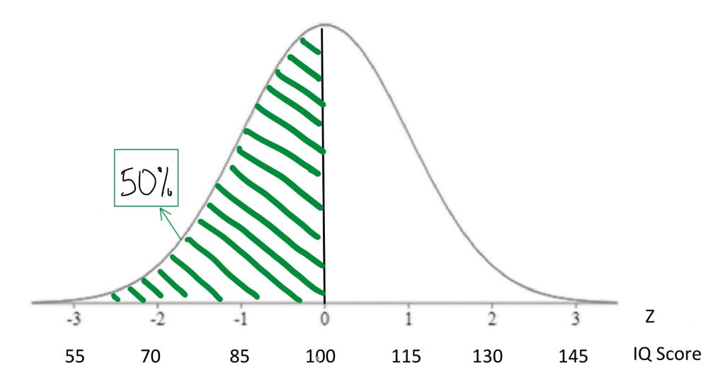
We saw that percentiles are expressions of area under a normal curve. Areas under the curve can be expressed as probability , too. For example, if we say the 50th percentile for IQ is 100, that can be expressed as: “If I chose a person at random, there is a 50% chance that they will have an IQ score below 100.”
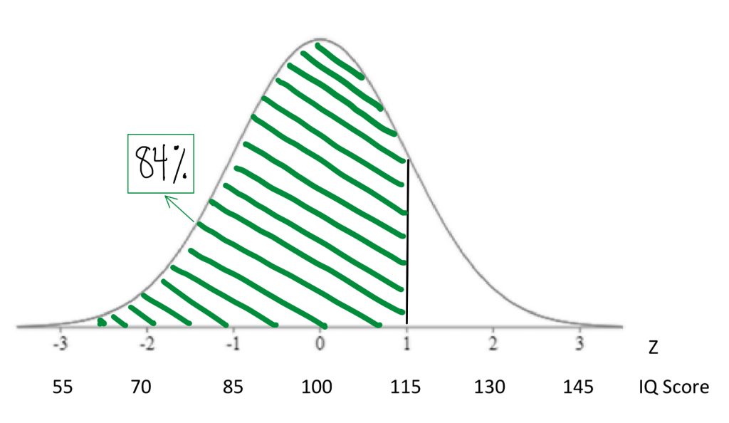
If we find the 84th percentile for IQ is 115 there is another way to say that “If I chose a person at random, there is an 84% chance that they will have an IQ score below 115.”
Concept Practice: find percentiles
Any time you are dealing with area under the normal curve, I encourage you to express that percentage in terms of probabilities . That will help you think clearly about what that area under the curve means once we get into the exercise of making decisions based on that information.
Concept Practice: interpreting percentile as probability
Probabilities , of course, range from 0 to 1 as proportions or fractions, and from 0% to 100% when expressed in percentage terms. In inferential statistics, we often express in terms of probability the likelihood that we would observe a particular score under a given normal curve model.
Concept Practice: applying probability
Although I encourage you to think of probabilities as percentages, the convention in statistics is to report to the probability of a score as a proportion, or decimal. The symbol used for “probability of score” is p . In statistics, the interpretation of “ p ” is a delicate subject. Generations of researchers have been lazy in our understanding of what “ p ”: tells us, and we have tended to over-interpret this statistic. As we begin to work with “ p ”, I will ask you to memorize a mantra that will help you report its meaning accurately. For now, just keep in mind that most psychologists and psychology students still make mistakes in how they express and understand the meaning of “ p ” values. This will take time and effort to fix, but I am confident that your generation will learn to do better at a precise and careful understanding of what statistics like “ p ” tell us… and what they do not.
To give you a sense of what a statement of p < .05 might mean, let us think back to our rat weights example.
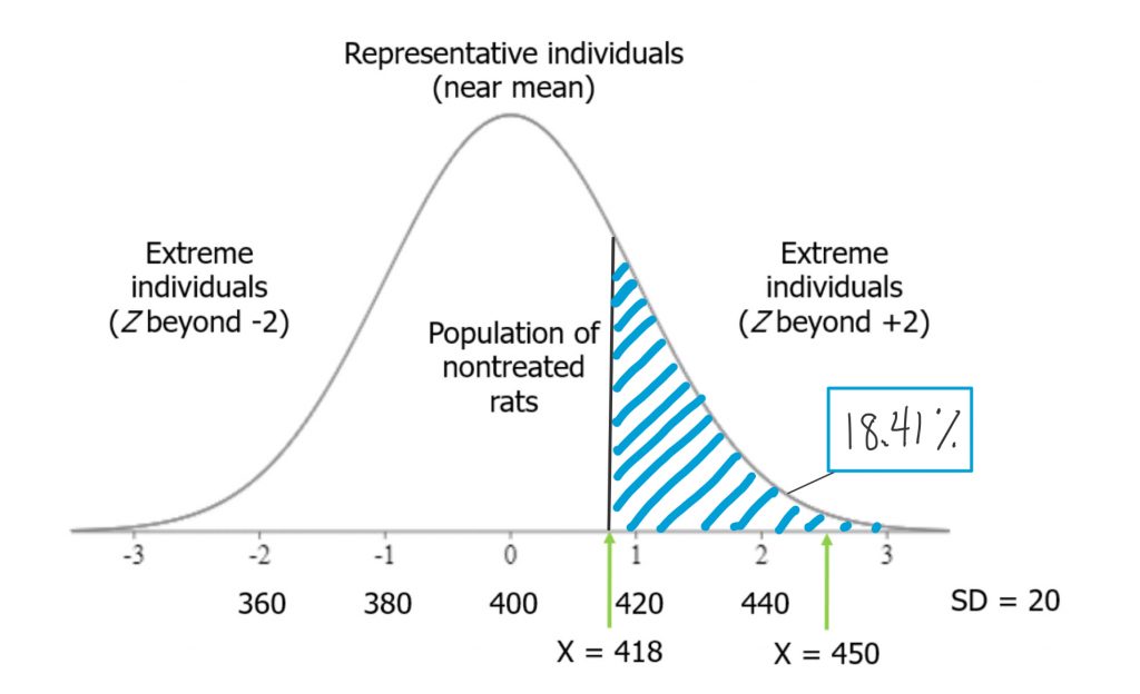
If I were to take a rat from our high-grain food group and place it on the distribution of untreated rat weights, and if it placed at Z = .9, we could look at the area under the curve from that point and above. That would tell us how likely it would be to observe such a heavy rat in the general population of nontreated rats — those that eat a normal diet.
Think of it this way. When we select a rat from our treatment group (those that ate the grain-heavy diet), and it is heavier than the average for a nontreated rat, there are two possible explanations for that observation. One is that the diet made him that way. As a scientist whose hypothesis is that a grain-heavy diet will make the rats weigh more, I’m actually motivated to interpret the observation that way. I want to believe this event is meaningful, because it is consistent with my hypothesis! But the other possibility is that, by random chance, we picked a rat that was heavy to begin with. There are plenty of rats in the distribution of nontreated rats that were at least that heavy. So there is always some probability that we just randomly selected a heavier rat. In this case, if my treated rat’s weight was less than one standard deviation above the mean, we saw in the chapter on normal curves that the probability of observing a rat weight that high or higher in the nontreated population was about 18%. That is not so unusual. It would not be terribly surprising if that outcome were simply the result of random chance rather than a result of the diet the rat had been eating.
If, on the other hand, the rat we measured was 2.5 standard deviations above the mean, the tail probability beyond that Z-score would be vanishingly small.
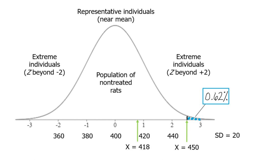
The probability of observing such a rat weight in the nontreated population is very low, so it is far less likely that observation can be accounted for just by random chance alone. As we accumulate more evidence, the probability they could have come at random from the nontreated population will weigh into our decision making about whether the grain-heavy diet indeed causes rats to become heavier. This is the way probabilities are used in the process of hypothesis testing , the logic of inferential statistics that we will look at soon.
Concept Practice: statistics as probability
Now that you have seen the relevance of probability to the decision making process that comprises inferential statistics, we have one more major learning objective: to become familiar with the central limit theorem .
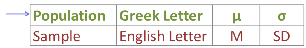
However, before we get to the central limit theorem , we need to be clear on the distinction between two concepts: sample and population . In the world of statistics, the population is defined as all possible individuals or scores about which we would ideally draw conclusions. When we refer to the characteristics, or parameters, that describe a population , we will use Greek letters. A sample is defined as the individuals or scores about which we are actually drawing conclusions. When we refer to the characteristics, or statistics, that describe a sample , we will use English letters.
It is important to understand the difference between a population and a sample , and how they relate to one another, in order to comprehend the central limit theorem and its usefulness for statistics. From a population we can draw multiple samples . The larger sample , the more closely our sample will represent the population .
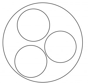
Think of a Venn diagram. There is a circle that is a population . Inside that large circle, you can draw an infinite number of smaller circles, each of which represents a sample .
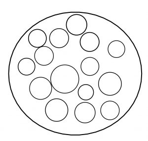
The larger that inner circle, the more of the population it contains, and thus the more representative it is.
Let us take a concrete example. A population might be the depression screening scores for all current postsecondary students in Canada. A sample from that population might be depression screening scores for 500 randomly selected postsecondary students from several institutions across Canada. That seems a more reasonable proportion of the two million students in the population than a sample that contains only 5 students. The 500 student sample has a better shot at adequately representing the entire population than does the 5 student sample , right? You can see that intuitively… and once you learn the central limit theorem , you will see the mathematical demonstration of the importance of sample size for representing the population .
To conduct the inferential statistics we are using in this course, we will be using the normal curve model to estimate probabilities associated with particular scores. To do that, we need to assume that data are normally distributed. However, in real life, our data are almost never actually a perfect match for the normal curve.
So how can we reasonably make the normality assumption? Here’s the thing. The central limit theorem is a mathematical principle that assures us that the normality assumption is a reasonable one as long as we have a decent sample size.
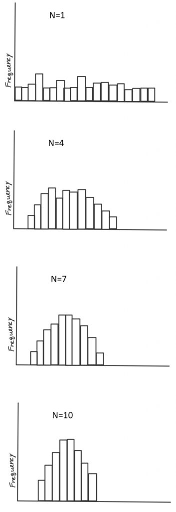
According to the theorem, as long as we take a decent-sized sample , if we took many samples (10,000) of large enough size (30+) and took the mean each time, the distribution of those means w ill approach a normal distribution, even if the scores from each sample are not normally distributed. To see this for yourself, take a look at the histograms shown on the right. The top histogram came from taking from a population 10,000 samples of just one score each, and plotting them on a histogram. See how it has a flat, or rectangular shape? No way we could call that a shape approximating a normal curve. Next is a histogram that came from taking the means of 10,000 samples , if each sample included 4 scores. Looks slightly better, but still not very convincing. With a sample size of 7, it looks a bit better. Once our sample size is 10, we at least have something pretty close. Mathematically speaking, as long as the sample size is no smaller than 30, then the assumption of normality holds. The other way we can reasonably make the normality assumption is if we know the population itself follows a normal curve. In that case, even if individual samples do not have a nice shaped histogram, that is okay, because the normality assumption is one apply to the population in question, not to the sample itself.
Now, you can play around with an online demonstration so you can really convince yourself that the central limit theorem works in practice. The goal here is to see what sample size is sufficient to generate a histogram that closely approximates a normal curve. And to trust that even if real-life data look wonky, the normal curve may still be a reasonable model for data analysis for purposes of inference.
Concept Practice: Central Limit Theorem
4b. hypothesis testing.
We are finally ready for your first introduction to a formal decision making procedure often used in statistics, known as hypothesis testing .
In this course, we started off with descriptive statistics, so that you would become familiar with ways to summarize the important characteristics of datasets. Then we explored the concepts standardizing scores, and relating those to probability as area under the normal curve model. With all those tools, we are now ready to make something!

Okay, not furniture, exactly, but decisions.
We are now into the portion of the course that deals with inferential statistics. Just to get you thinking in terms of making decisions on the basis of data, let us take a slightly silly example. Suppose I have discovered a pill that cures hangovers!

Well, it greatly lessened symptoms of hangover in 10 of the 15 people I tested it on. I am charging 50 dollars per pill. Will you buy it the next time you go out for a night of drinking? Or recommend it to a friend? … If you said yes, I wonder if you are thinking very critically? Should we think about the cost-benefit ratio here on the basis of what information you have? If you said no, I bet some of the doubts I bring up popped to your mind as well. If 10 out of 15 people saw lessened symptoms, that’s 2/3 of people – so some people saw no benefits. Also, what does “greatly lessened symptoms of hangover” mean? Which symptoms? How much is greatly? Was the reduction by two or more standard deviations from the mean? Or was it less than one standard deviation improvement? Given the cost of 50 dollars per pill, I have to say I would be skeptical about buying it without seeing some statistics!
On this list is a preview of the basic concepts to which you will be introduced as we go through the rest of this chapter.
Hypothesis Testing Basic Concepts
- Null Hypothesis
- Research Hypothesis (alternative hypothesis)
- Statistical significance
- Conventional levels of significance
- Cutoff sample score (critical value)
- Directional vs. non-directional hypotheses
- One-tailed and two-tailed tests
- Type I and Type II errors
You can see that there are lots of new concepts to master. In my experience, each concept makes the most sense in context, within its place in the hypothesis testing workflow. We will start with defining our null and research hypotheses , then discuss the levels of statistical significance and their conventional usage. Next, we will look at how to find the cutoff sample score that will form the critical value for our decision criterion. We will look at how that differs for directional vs. non-directional hypotheses , which will lend themselves to one- or two-tailed tests , respectively.
The hypothesis testing procedure, or workflow, can be broken down into five discrete steps.
Steps of Hypothesis Testing
- Restate question as a research hypothesis and a null hypothesis about populations.
- Determine characteristics of the comparison distribution.
- Determine the cutoff sample score on the comparison distribution at which the null hypothesis should be rejected.
- Determine your sample’s score on the comparison distribution.
- Decide whether to reject the null hypothesis.
These steps are something we will be using pretty much the rest of the semester, so it is worth memorizing them now. My favourite approach to that is to create a mnemonic device. I recommend the following key words from which to form your mnemonic device: hypothesis, characteristics, cutoff, score, and decide. Not very memorable? Try association those with more memorable words that start with the same letter or sound. How about “ Happy Chickens Cure Sad Days .” Or you can put the words into a mnemonic device generator on the internet and get something truly bizarre. I just tried one and got “ Hairless Carsick Chewbacca Slapped Demons ”. Another good one: “ Hamlet Chose Cranky Sushi Drunkenly .” Anyway, you play around with it or brainstorm until you hit upon one that works for you. Who knew statistics could be this much fun!
The first step in hypothesis testing is always to formulate hypotheses. The first rule that will help you do so correctly, is that hypotheses are always about populations . We study samples in order to make conclusions about populations, so our predictions should be about the populations themselves. First, we define population 1 and population 2. Population 1 is always defined as people like the ones in our research study, the ones we are truly interested in. Population 2 is the comparison population , the status quo to which we are looking to compare our research population . Now, remember, when referring to populations , we always use Greek letters. So if we formulate our hypotheses in symbols, we need to use Greek letters.
It is a good idea to state our hypotheses both in symbols and in words. We need to make them specific and disprovable. If you follow my tips, you will have it down with just a little practice.
We need to state two hypotheses. First, we state the research hypothesis , which is sometimes referred to as the alternative hypothesis. The research hypothesis (often called the alternative hypothesis) is a statement of inequality, or that Something happened! This hypothesis makes the prediction that the population from which the research sample came is different from the comparison population . In other words, there is a really high probability that the sample comes from a different distribution than the comparison one.
The null hypothesis , on the other hand, is a statement of equality, or that nothing happened. This hypothesis makes the prediction that the population from which sample came is not different from the comparison population . We set up the null hypothesis as a so-called straw man, that we hope to tear down. Just remember, null means nothing – that nothing is different between the populations .
Step two of hypothesis testing is to determine the characteristics of the comparison distribution. This is where our descriptive statistics, the mean and standard deviation, come in. We need to ensure our normal curve model to which we are comparing our research sample is mapped out according to the particular characteristics of the population of comparison, which is population 2.
Next it is time to set our decision rule. Step 3 is to determine the cutoff sample score , which is derived from two pieces of information. The first is the conventional significance level that applies. By convention, the probability level that we are willing to accept as a risk that the score from our research sample might occur by random chance within the comparison distribution is set to one of three levels: 10%, 5%, or 1%. The most common choice of significance level is 5%. Typically the significance level will be provided to you in the problem for your statistics courses, but if it is not, just default to a significance level of .05. Sometimes researchers will choose a more conservative significance level , like 1%, if they are particularly risk averse. If the researcher chooses a 10% significance level , they are likely conducting a more exploratory study, perhaps a pilot study, and are not too worried about the probability that the score might be fairly common under the comparison distribution.
The second piece of information we need to know in order to find our cutoff sample score is which tail we are looking at. Is this a directional hypothesis , and thus one-tailed test ? Or a non-directional hypothesis , and thus a two-tailed test ? This depends on the research hypothesis from step 1. Look for directional keywords in the problem. If the researcher prediction involves words like “greater than” or “larger than”, this signals that we should be doing a one-tailed test and that our cutoff sample score should be in the top tail of the distribution. If the researcher prediction involves words like “lower than” or “smaller than”, this signals that we should be doing a one-tailed test and that our cutoff sample score should be in the bottom tail of the distribution. If the prediction is neutral in directionality, and uses a word like “different”, that signals a non-directional hypothesis . In that case, we would need to use a two-tailed test, and our cutoff scores would need to be indicated on both tails of the distribution. To do that, we take our area under the curve, which matches our significance level , and split it into both tails.
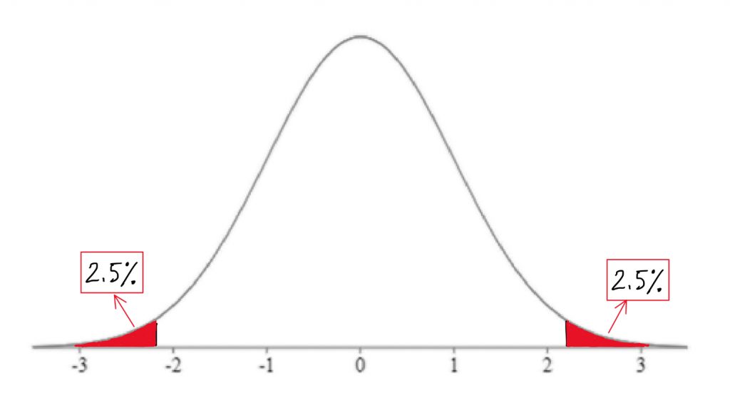
For example, if we have a two-tailed test with a .05 significance level , then we would split the 5% area under the curve into the two tails, so two and a half percent in each tail.
Concept Practice: deciding on one-tailed vs. two-tailed tests
We can find the Z-score that forms the border of the tail area we have identified based on significance level and directionality by looking it up in a table or an online calculator . I always recommend mapping this cutoff score onto a drawing of the comparison distribution as shown above. This should help you visualize the setup of the hypothesis test clearly and accurately.
Concept Practice: inference through hypothesis testing
The next step in the hypothesis testing procedure is to determine your sample’s score on the comparison distribution. To do this, we calculate a test statistic from the sample raw score, mark it on the comparison distribution, and determine whether it falls in the shaded tail or not. In reality, we would always have a sample with more than one score in it. However, for the sake of keeping our test statistic formula a familiar one, we will use a sample size of one. We will use our Z-score formula to translate the sample’s raw score into a Z-score – in other words, we will figure out how many standard deviations above or below the comparison distribution’s mean the sample score is.
![\[Z=\frac{X-M}{SD}\]](https://pressbooks.bccampus.ca/statspsych/wp-content/ql-cache/quicklatex.com-9ff4a1c7099641ee0b6856dfdc537f34_l3.png "Rendered by QuickLaTeX.com")
Finally, it’s time to decide whether to reject the null hypothesis . This decision is based on whether our sample’s data point was more extreme than the cutoff score , in other words, “did it fall in the shaded tail?” If the sample score is more extreme than the cutoff score , then we must reject the null hypothesis. Our research hypothesis is supported! (Not proven… remember, there is still some probability that that score could have occurred randomly within the comparison distribution.) But it is sound to say that it appears quite likely that the population from which our sample came is different from the comparison population. Another way to express this decision is to say that the result was statistically significant , which is to say that there is less than a 5% chance of this result occurring randomly within the comparison distribution (here I just filled in the blank with the significance level).
What if the research sample score did not fall in the shaded tail? In the case that the sample score is less extreme than the cutoff score , then our research hypothesis is not supported. We do not reject the null hypothesis . It appears that the population from which our sample came is not different from the comparison population . Note that we do not typically express this result as “accept the null hypothesis” or “we have proved the null hypothesis”. From this test, we do not have evidence that the null hypothesis is correct, rather we simply did not have enough evidence to reject it. Another way to express this decision is to say that the result was not statistically significant , which is to say that there is more than a 5% chance of this result occurring randomly within the comparison distribution (here I just used the most common significance level ).
Concept Practice: interpreting conclusions of hypothesis tests
So we have described the hypothesis testing process from beginning to end. The whole process of null hypothesis testing can feel like pretty tortured logic at first. So let us zoom out, and look at the whole process another way. Essentially what we are seeking to do in such a hypothesis test is to compare two populations . We want to find out if the populations are distinct enough to confidently state that there is a difference between population 1 and population 2. In our example, we wanted to know if the population of people using a new medication, population 1, sleep longer than the population of people who are not using that new medication, population 2. We ended up finding that the research evidence to hand suggests population 1’s distribution is distinct enough from population 2 that we could reject the null hypothesis of similarity.
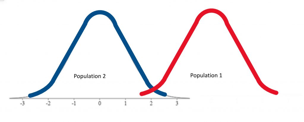
In other words, we were able to conclude that the difference between the centres of the two distributions was statistically significant .
If, on the other hand, the distributions were a bit less distinct, we would not have been able to make that claim of a significant difference.
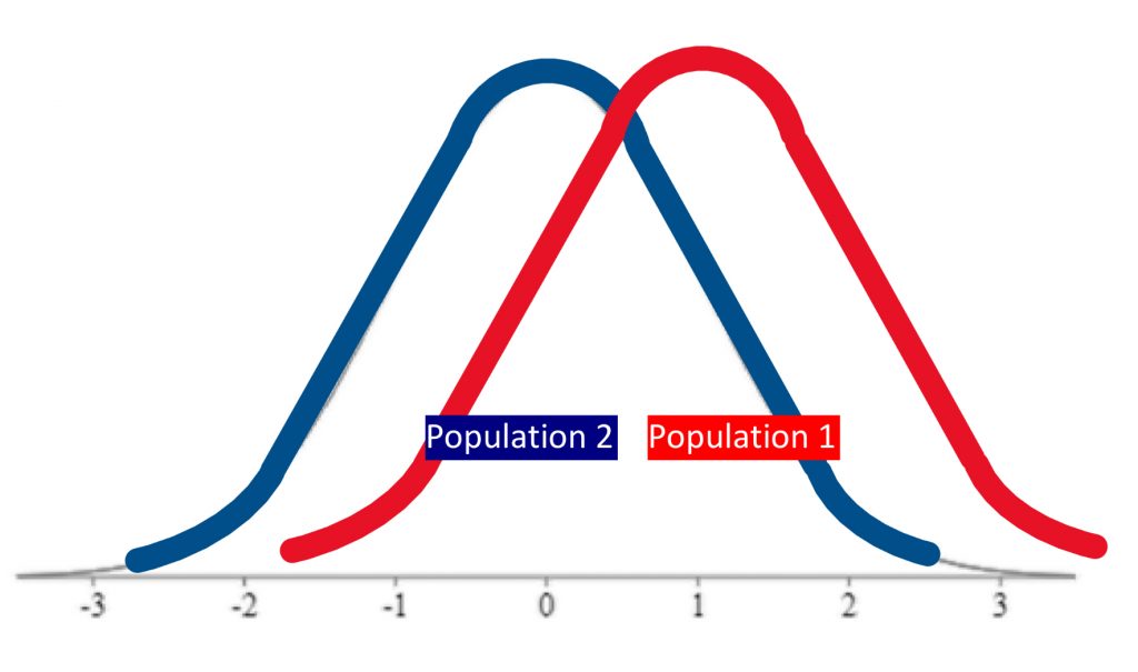
We would not have rejected the null hypothesis if evidence indicated the populations were too similar.
Just how different do the two distributions need to be? That criterion is set by the cutoff score , which depends on the significance level , and whether it is a one-tailed or two-tailed hypothesis test .
Concept Practice: Putting hypothesis test elements together
That was a lot of new concepts to take on! As a reward, assuming you enjoy memes, there are a plethora of statistics memes , some of which you may find funny now that you have made it into inferential statistics territory. Welcome to the exclusive club of people who have this rather peculiar sense of humour. Enjoy!
Chapter Summary
In this chapter we examined probability and how it can be used to make inferences about data in the framework of hypothesis testing . We now have a sense of how two populations can be compared and the difference between their means evaluated for statistical significance .
Concept Practice
Return to text.
Return to 4a. Probability and Inferential Statistics
Try interactive Worksheet 4a or download Worksheet 4a
Return to 4b. Hypothesis Testing
Try interactive Worksheet 4b or download Worksheet 4b
in a situation where several different outcomes are possible, the probability of any specific outcome is a fraction or proportion of all possible outcomes
mathematical theorem that proposes the following: as long as we take a decent-sized sample, if we took many samples (10,000) of large enough size (30+) and took the mean each time, the distribution of those means will approach a normal distribution, even if the scores from each sample are not normally distributed
all possible individuals or scores about which we would ideally draw conclusions
a formal decision making procedure often used in inferential statistics
the individuals or scores about which we are actually drawing conclusions
the probability level that we are willing to accept as a risk that the score from our research sample might occur by random chance within the comparison distribution. By convention, it is set to one of three levels: 10%, 5%, or 1%.
critical value that serves as a decision criterion in hypothesis testing
prediction that the population from which the research sample came is different from the comparison population
the prediction that the population from which sample came is not different from the comparison population
a research prediction that the research population mean will be “greater than” or "less than" the comparison population mean
a hypothesis test in which there is only one cutoff sample score on either the lower or the upper end of the comparison distribution
a research prediction that the research population mean will be “different from" the comparison population mean, but allows for the possibility that the research population mean may be either greater than or less than the comparison population mean
a hypothesis test in which there are two cutoff sample scores, one on either end of the comparison distribution
a decision in hypothesis testing that concludes statistical significance because the sample score is more extreme than the cutoff score
the conclusion from a hypothesis test that probability of the observed result occurring randomly within the comparison distribution is less than the significance level
a decision in hypothesis testing that is inconclusive because the sample score is less extreme than the cutoff score
Beginner Statistics for Psychology Copyright © 2021 by Nicole Vittoz is licensed under a Creative Commons Attribution-NonCommercial 4.0 International License , except where otherwise noted.
- Skip to secondary menu
- Skip to main content
- Skip to primary sidebar
Statistics By Jim
Making statistics intuitive
Normal Distribution in Statistics
By Jim Frost 181 Comments
The normal distribution, also known as the Gaussian distribution, is the most important probability distribution in statistics for independent, random variables. Most people recognize its familiar bell-shaped curve in statistical reports.
The normal distribution is a continuous probability distribution that is symmetrical around its mean, most of the observations cluster around the central peak, and the probabilities for values further away from the mean taper off equally in both directions. Extreme values in both tails of the distribution are similarly unlikely. While the normal distribution is symmetrical, not all symmetrical distributions are normal. For example, the Student’s t, Cauchy, and logistic distributions are symmetric.
As with any probability distribution, the normal distribution describes how the values of a variable are distributed. It is the most important probability distribution in statistics because it accurately describes the distribution of values for many natural phenomena. Characteristics that are the sum of many independent processes frequently follow normal distributions. For example, heights, blood pressure, measurement error, and IQ scores follow the normal distribution.
In this blog post, learn how to use the normal distribution, about its parameters, the Empirical Rule, and how to calculate Z-scores to standardize your data and find probabilities.
Example of Normally Distributed Data: Heights
Height data are normally distributed. The distribution in this example fits real data that I collected from 14-year-old girls during a study. The graph below displays the probability distribution function for this normal distribution. Learn more about Probability Density Functions .

As you can see, the distribution of heights follows the typical bell curve pattern for all normal distributions. Most girls are close to the average (1.512 meters). Small differences between an individual’s height and the mean occur more frequently than substantial deviations from the mean. The standard deviation is 0.0741m, which indicates the typical distance that individual girls tend to fall from mean height.
The distribution is symmetric. The number of girls shorter than average equals the number of girls taller than average. In both tails of the distribution, extremely short girls occur as infrequently as extremely tall girls.
Parameters of the Normal Distribution
As with any probability distribution, the parameters for the normal distribution define its shape and probabilities entirely. The normal distribution has two parameters, the mean and standard deviation. The Gaussian distribution does not have just one form. Instead, the shape changes based on the parameter values, as shown in the graphs below.
The mean is the central tendency of the normal distribution. It defines the location of the peak for the bell curve. Most values cluster around the mean. On a graph, changing the mean shifts the entire curve left or right on the X-axis. Statisticians denote the population mean using μ (mu).
μ is the expected value of the normal distribution. Learn more about Expected Values: Definition, Using & Example .

Related posts : Measures of Central Tendency and What is the Mean?
Standard deviation σ
The standard deviation is a measure of variability. It defines the width of the normal distribution. The standard deviation determines how far away from the mean the values tend to fall. It represents the typical distance between the observations and the average. Statisticians denote the population standard deviation using σ (sigma).
On a graph, changing the standard deviation either tightens or spreads out the width of the distribution along the X-axis. Larger standard deviations produce wider distributions.

When you have narrow distributions, the probabilities are higher that values won’t fall far from the mean. As you increase the spread of the bell curve, the likelihood that observations will be further away from the mean also increases.
Related post : Measures of Variability and Standard Deviation
Population parameters versus sample estimates
The mean and standard deviation are parameter values that apply to entire populations. For the Gaussian distribution, statisticians signify the parameters by using the Greek symbol μ (mu) for the population mean and σ (sigma) for the population standard deviation.
Unfortunately, population parameters are usually unknown because it’s generally impossible to measure an entire population. However, you can use random samples to calculate estimates of these parameters. Statisticians represent sample estimates of these parameters using x̅ for the sample mean and s for the sample standard deviation.
Learn more about Parameters vs Statistics: Examples & Differences .
Common Properties for All Forms of the Normal Distribution
Despite the different shapes, all forms of the normal distribution have the following characteristic properties.
- They’re all unimodal , symmetric bell curves. The Gaussian distribution cannot model skewed distributions.
- The mean, median, and mode are all equal.
- Half of the population is less than the mean and half is greater than the mean.
- The Empirical Rule allows you to determine the proportion of values that fall within certain distances from the mean. More on this below!
While the normal distribution is essential in statistics, it is just one of many probability distributions, and it does not fit all populations. To learn how to determine whether the normal distribution provides the best fit to your sample data, read my posts about How to Identify the Distribution of Your Data and Assessing Normality: Histograms vs. Normal Probability Plots .
The uniform distribution also models symmetric, continuous data, but all equal-sized ranges in this distribution have the same probability, which differs from the normal distribution.
If you have continuous data that are skewed, you’ll need to use a different distribution, such as the Weibull , lognormal , exponential , or gamma distribution.
Related post : Skewed Distributions
The Empirical Rule for the Normal Distribution
When you have normally distributed data, the standard deviation becomes particularly valuable. You can use it to determine the proportion of the values that fall within a specified number of standard deviations from the mean. For example, in a normal distribution, 68% of the observations fall within +/- 1 standard deviation from the mean. This property is part of the Empirical Rule, which describes the percentage of the data that fall within specific numbers of standard deviations from the mean for bell-shaped curves.
| 1 | 68% |
| 2 | 95% |
| 3 | 99.7% |
Let’s look at a pizza delivery example. Assume that a pizza restaurant has a mean delivery time of 30 minutes and a standard deviation of 5 minutes. Using the Empirical Rule, we can determine that 68% of the delivery times are between 25-35 minutes (30 +/- 5), 95% are between 20-40 minutes (30 +/- 2*5), and 99.7% are between 15-45 minutes (30 +/-3*5). The chart below illustrates this property graphically.

If your data do not follow the Gaussian distribution and you want an easy method to determine proportions for various standard deviations, use Chebyshev’s Theorem ! That method provides a similar type of result as the Empirical Rule but for non-normal data.
To learn more about this rule, read my post, Empirical Rule: Definition, Formula, and Uses .
Standard Normal Distribution and Standard Scores
As we’ve seen above, the normal distribution has many different shapes depending on the parameter values. However, the standard normal distribution is a special case of the normal distribution where the mean is zero and the standard deviation is 1. This distribution is also known as the Z-distribution.
A value on the standard normal distribution is known as a standard score or a Z-score. A standard score represents the number of standard deviations above or below the mean that a specific observation falls. For example, a standard score of 1.5 indicates that the observation is 1.5 standard deviations above the mean. On the other hand, a negative score represents a value below the average. The mean has a Z-score of 0.

Suppose you weigh an apple and it weighs 110 grams. There’s no way to tell from the weight alone how this apple compares to other apples. However, as you’ll see, after you calculate its Z-score, you know where it falls relative to other apples.
Learn how the Z Test uses Z-scores and the standard normal distribution to determine statistical significance.
Standardization: How to Calculate Z-scores
Standard scores are a great way to understand where a specific observation falls relative to the entire normal distribution. They also allow you to take observations drawn from normally distributed populations that have different means and standard deviations and place them on a standard scale. This standard scale enables you to compare observations that would otherwise be difficult.
This process is called standardization, and it allows you to compare observations and calculate probabilities across different populations. In other words, it permits you to compare apples to oranges. Isn’t statistics great!
To standardize your data, you need to convert the raw measurements into Z-scores.
To calculate the standard score for an observation, take the raw measurement, subtract the mean, and divide by the standard deviation. Mathematically, the formula for that process is the following:
X represents the raw value of the measurement of interest. Mu and sigma represent the parameters for the population from which the observation was drawn.
After you standardize your data, you can place them within the standard normal distribution. In this manner, standardization allows you to compare different types of observations based on where each observation falls within its own distribution.
Example of Using Standard Scores to Make an Apples to Oranges Comparison
Suppose we literally want to compare apples to oranges. Specifically, let’s compare their weights. Imagine that we have an apple that weighs 110 grams and an orange that weighs 100 grams.
If we compare the raw values, it’s easy to see that the apple weighs more than the orange. However, let’s compare their standard scores. To do this, we’ll need to know the properties of the weight distributions for apples and oranges. Assume that the weights of apples and oranges follow a normal distribution with the following parameter values:
| Mean weight grams | 100 | 140 |
| Standard Deviation | 15 | 25 |
Now we’ll calculate the Z-scores:
- Apple = (110-100) / 15 = 0.667
- Orange = (100-140) / 25 = -1.6
The Z-score for the apple (0.667) is positive, which means that our apple weighs more than the average apple. It’s not an extreme value by any means, but it is above average for apples. On the other hand, the orange has fairly negative Z-score (-1.6). It’s pretty far below the mean weight for oranges. I’ve placed these Z-values in the standard normal distribution below.

While our apple weighs more than our orange, we are comparing a somewhat heavier than average apple to a downright puny orange! Using Z-scores, we’ve learned how each fruit fits within its own bell curve and how they compare to each other.
For more detail about z-scores, read my post, Z-score: Definition, Formula, and Uses
Finding Areas Under the Curve of a Normal Distribution
The normal distribution is a probability distribution. As with any probability distribution, the proportion of the area that falls under the curve between two points on a probability distribution plot indicates the probability that a value will fall within that interval. To learn more about this property, read my post about Understanding Probability Distributions .
Typically, I use statistical software to find areas under the curve. However, when you’re working with the normal distribution and convert values to standard scores, you can calculate areas by looking up Z-scores in a Standard Normal Distribution Table.
Because there are an infinite number of different Gaussian distributions, publishers can’t print a table for each distribution. However, you can transform the values from any normal distribution into Z-scores, and then use a table of standard scores to calculate probabilities.
Using a Table of Z-scores
Let’s take the Z-score for our apple (0.667) and use it to determine its weight percentile. A percentile is the proportion of a population that falls below a specific value. Consequently, to determine the percentile, we need to find the area that corresponds to the range of Z-scores that are less than 0.667. In the portion of the table below, the closest Z-score to ours is 0.65, which we’ll use.

Click here for a full Z-table and illustrated instructions for using it !
The trick with these tables is to use the values in conjunction with the properties of the bell curve to calculate the probability that you need. The table value indicates that the area of the curve between -0.65 and +0.65 is 48.43%. However, that’s not what we want to know. We want the area that is less than a Z-score of 0.65.
We know that the two halves of the normal distribution are mirror images of each other. So, if the area for the interval from -0.65 and +0.65 is 48.43%, then the range from 0 to +0.65 must be half of that: 48.43/2 = 24.215%. Additionally, we know that the area for all scores less than zero is half (50%) of the distribution.
Therefore, the area for all scores up to 0.65 = 50% + 24.215% = 74.215%
Our apple is at approximately the 74 th percentile.
Below is a probability distribution plot produced by statistical software that shows the same percentile along with a graphical representation of the corresponding area under the bell curve. The value is slightly different because we used a Z-score of 0.65 from the table while the software uses the more precise value of 0.667.

Related post : Percentiles: Interpretations and Calculations
Other Reasons Why the Normal Distribution is Important
In addition to all of the above, there are several other reasons why the normal distribution is crucial in statistics.
- Some statistical hypothesis tests assume that the data follow a bell curve. However, as I explain in my post about parametric and nonparametric tests , there’s more to it than only whether the data are normally distributed.
- Linear and nonlinear regression both assume that the residuals follow a Gaussian distribution. Learn more in my post about assessing residual plots .
- The central limit theorem states that as the sample size increases, the sampling distribution of the mean follows a normal distribution even when the underlying distribution of the original variable is non-normal.
That was quite a bit about the bell curve! Hopefully, you can understand that it is crucial because of the many ways that analysts use it.
If you’re learning about statistics and like the approach I use in my blog, check out my Introduction to Statistics book! It’s available at Amazon and other retailers.

Share this:

Reader Interactions

January 17, 2023 at 8:55 am
Thanks Jim for the detailed response. much appreciated.. it makes sense.
January 16, 2023 at 7:20 pm
Hi Jim, well, one caveat to your caveat. 🙂 I am assuming that even though we know the general mean is 100, that we do NOT know if there is something inherent about the two schools whereby their mean might not represent the general population, in fact I made it extreme to show that their respective means are probably NOT 100.. So, for the school with an IQ of 60, maybe it is 100, maybe it is 80, maybe it is 60, maybe it is 50, etc. But it seems to me that we could do a probability distribution around each of those in some way. (i.e what if their real mean was 100, what is the sampling distribution, what if the real mean is 80, what is the samplind distribution, etc.) So, I guess ultimately, I am asking two things. 1) what is the real mean for the school with a mean of 60 (in the case of the lower scoring school-intuition tells me it must be higher), but the second question then is, and perhaps the real crux of my question is how would we go about estimating those respective means. To me, this has Bayesian written all over it (the prior is 100, the updated info is 60, etc). But I only know Bayes with probabilities. anyway, I think this is an important question with bayesian thinking needed, and I dont think this subject gets the attention it deserves. I much appreciate your time, Jim. Hopefully a hat trick (3rd response) will finish this up. 🙂 — and hopefully your readers get something from this. Thanks John

January 16, 2023 at 11:08 pm
I explicitly mentioned that as an assumption in my previous comment. The schools need to represent the general population in terms of its IQ score distribution. Yes, it’s possible that the schools represent a different population. In that case, the probabilities don’t apply AND you wouldn’t even know whether the subsequent sample mean was likely to be higher or lower. You’d need to do a bit investigation to determine whether the school represented the general population or some other population. That’s exactly why I mentioned that. And my answer was based on you wanting to use the outside knowledge of the population.
Now, if you don’t want to assume that the general population’s IQ distribution is a normal distribution with a mean of 100 and standard deviation of 15, then you’re back to what I was writing about in my previous comment where you don’t use that information. In short, if you want to know the school’s true mean IQ, you’ll need to treat it as your population. Then draw a good sized random sample from it. Or, if the school is small enough, assess the entire school. As it is, you only have a sample size of 5. That’s not going to give you a precise estimate. You’d check the confidence interval for that estimate to see a range of likely values for the school’s mean.
You could use a Bayesian approach. That’s not my forte. But if you did draw a random sample of 5 and got a mean IQ of 60, that’s so unlikely to occur if the school’s mean is 100 that using a prior of 100 in a Bayesian analysis is questionable. That’s the problem with Bayesian approaches. You need priors, for which you don’t always have solid information. In your example, you’d need to know a lot more about the schools to have reasonable priors.
In this case, it seems likely that the schools mean IQ is not 100. It’s probably lower, but what is it. Hard to say. Seems like you’d need to really investigate the school to see what’s going on. Did you just get a really flukey sample, but the school does represent the general population. Or, does the school represent a different population?
Until you really looked in-depth at the school to get at that information, your best estimate is your sample mean along with the CI to understand its low precision.
January 16, 2023 at 9:54 am
Hi Jim, Thanks for response. I was assuming that we DO KNOW it has a general population mean of 100. I was also thinking in a Bayesian way that knowing the general population mean is 100, that the REAL Mean of the one school is BETWEEN 60 and 100 and the REAL mean of the other school is BETWEEN 100 and 140, much like if you were a baseball scout and you know that the average player is a .260 hitter, and you watch him bat 10 times, and get 8 hits, you would not assume his REAL ability is .800, you would assume it is BETWEEN .260 and .800 and perhaps use a Beta distribution, to conclude his distribution of averages is centered, at.. I don’t know, something like .265… something LARGER than .260. But this seems paradoxical to the idea that if we did get a sample of 5 (or however, many) and got a mean of 60 and in thinking of a confidence interval for that mean of 60, it is equally like that the REAL mean is say 55 as compared to 65.
January 16, 2023 at 6:50 pm
Gotcha! So, yes, using the knowledge outside our dataset, we can draw some additional conclusions.
For one thing, there’s regression to the mean. Usually that applies to one unusual observation being followed by an observation that is likely to be closer to the mean. In this case, we can use the same principle but apply it to samples of N = 5. You’ve got an unusual sample from each school. If you were to draw another random sample of the same size from each school, those samples are likely to be closer to the mean.
There are a few caveats. We’re assuming that we’re drawing random samples and that the schools reflect the general population rather than special populations.
As for getting the probability for N = 5 of the IQ sample mean equaling 60 or 140, we can use the sampling distribution as I mentioned. We need to find the probability of obtaining a random sample 140. The graph shows the sampling distribution below.

The probability for 140 is the same. Total probability getting either condition in one random sample is 0.0000000024788.
As you can see, either probability is quite low! Basically, don’t count on getting either sample mean under these conditions! Those sample means are just far out in the tails of the sampling distribution.
But, if you did get either of those means, what’s the probability that the next random sample of N = 5 will be closer to the true mean?
That probability equals: 1 – 0.0000000024788 = 0.9999999975212
It’s virtually guaranteed in this case that the next random sample of 5 will be closer to the correct mean!
January 13, 2023 at 8:11 am
Hi Jim, Thanks for these posts. I have a question related to the error term in a normal distribution. Let’s assume that we are taking IQs at various high schools. we go to one high school, take 5 IQ’s and the mean is 140. we go to another, take 5 IQS and the mean is 60. We are trying to determine the population mean at each school. Of course, We know that the 140 and 60 are just estimates of the respective high schools, is there some “boundedness” concept (seems intuitive) that would suggest that the real mean at the one school is more likely higher than 60 than lower, and the mean at the other school is more likely lower than 140 than higher. I am thinking of a probability density function of error terms about each of 60 and 140 would illustrate that. Can we confirm this mathematically? hope my question makes sense. Thanks John
January 13, 2023 at 11:54 pm
That’s kind of a complex question! In the real world, we know that IQs are defined as having a general population mean of 100. But let’s pretend we don’t know that.
I’ll assume that you randomly sampled the 5 students at both of the schools.
Going strictly by the data we gathered, it would be hard for us to know whether the overall HS population mean is between the two schools. It’s also possible that the two high schools have different means for reasons unknown to us. So, it’s really hard to draw conclusions. Particularly with only a measly 5 observations at two schools. There’s going to be a large margin of uncertainty with both estimates.
So, we’ll left in a situation where we don’t know what the overall population mean is, we don’t know if the two high schools should have different means or not, and the two estimates we have wide margins of error.
In short, we don’t know much! What we should do over time is build our knowledge in this area. Get large samples from those two schools and other schools. Try to identify reasons why the IQs might be different at various schools. Or find that they should be nearly identical. After we build up our knowledge, we can help that aid our understanding.
But with just 5 observations at two schools and ignoring our real-world knowledge, we couldn’t put much faith in the estimates of 60 and 140 and really not much reason to assume the 60 should be higher and the 140 lower.
Now, if you want to apply real-world knowledge that we do have, yes, we can be reasonably sure that the 60 is too low and the 140 is too high. It is inconceivable that any reasonably sized school would have either mean for the entire school population unless they were schools intended for special students. It is much more likely that those are fluky samples based on the tiny sample size. We can know all that because we know that the population average truly is 100 with a standard deviation of 15. Given that fact, you could look at the sampling distribution of the mean for each school’s size to determine the probability of having such an extreme mean IQ for the entire school.
But it wasn’t clear from your question if you wanted to incorporate that information or not. If you do, then what you need is the sampling distribution of the mean and use that to calculate the probability for each school. It won’t tell you for sure whether the means are too high or too low, but you’ll see how unlikely they are to occur given the known properties of the population, and you could conclude it’s more likely they’re just wrong–too low and too high!

December 2, 2022 at 2:44 pm
Hello. I’m new to this field and have a very basic question. If the average number of engine hours on a small aircraft between oil services is 29.9. And my SD is 14.1, does that mean 68.27% of all values lie between 44.0 (29.9+14.1) and 15.8 (29.9-14.1)?
December 2, 2022 at 5:12 pm
You do need to assume or know that the distribution in question follows a normal distribution. If it does, then, yes, your conclusions are absolutely correct!
In statistics classes, you’ll frequently have questions that state you can assume the data follow a normal distribution or that it’s been determined that they do. In the real world, you’ll need previous research to establish that. Or you might use it as a rough estimate if you’re not positive about normality but pretty sure the distribution is at least roughly normal.
So, there are a few caveats but yes, you’re understanding is correct.

June 27, 2022 at 1:38 pm
Hello, I have a question related to judgments regarding a population and the potential to identify a mixture distribution. I have a dataset which is not continuous – there is a significant gap between two groups of data. Approximately 98% of my data is described by one group and 2% of my data by another group. The CDF of all data looks like a mixture distribution; there is a sharp change in local slopes on either side of the non-continuous data range. I am using NDE methods to detect residual stress levels in pipes. My hypothesis is that discrete stress levels exist as a result of manufacturing methods. That is, you either have typical stress levels or you have atypical stress levels. 1. Can the non-continuous nature of the data suggest a mixture distribution? 2. What test(s) can be performed to establish that the two sub-groups are not statistically compatible?

December 20, 2021 at 10:10 am
Thanks for how to identify what distribution to use. I was condused at first I have understoot in normal, it is continuous and w ecan see on the X -axis the SD line is not clossed on it. In the Poison, it is a discreet thus with a time frame/linit. In Binomial, the outcome expected is post/neg, yes/no, gfalse/true etc. Thus two outcomes.
I can also say that in normal , there is complexity in random variables to be used.
December 21, 2021 at 1:03 am
Hi Evalyne,
I’m not sure that I understand what your question is. Yes, normal distributions require continuous data. However, not all continuous data follow a normal distribution.
Poisson distributions use discrete data–specifically count data. Other types of discrete data do not follow the Poisson distribution. For more information, read about the Poisson distribution .
Binomial distributions model the expected outcomes for binary data. Read more about the binomial distribution .
December 20, 2021 at 10:00 am
Thanks Jim Frost for your resource. I am learning this and has added alot to my knowledge.

November 15, 2021 at 2:44 pm
Thanks for your explanations, they are very helpful

October 5, 2021 at 4:21 am
Interesting. I Need help. Lets say I have 5 columns A B C D E
A follows Poisson Distribution B follows Binomial Distribution C follows Weibull Distribution D follows Negative Binomial Distribution E follows Exponential Distribution
Alright now I know what type of distribution my data follows, Then What should I do next ? How can this help me in exploratory data analysis ,in decision making or in machine learning ?
What if I don’t know what type of distribution my data follows because they all look confusing or similar when plotting it. Is there any equation can help ? is there libraries help me identifies the probability distribution of the data ?
Kindly help
October 7, 2021 at 11:50 pm
Hi Savitur,
There are distribution tests that will help you identify the distribution that best fits your data. To learn how to do that, read my post about How to Identify the Distribution of Your Data .
After you know the distribution, you can use it to make better predictions, estimate probabilities and percentiles, etc.

June 17, 2021 at 2:25 pm
Jim, Simple question. I am working on a regression analysis to determine which of many variables predict success in nursing courses. I had hoped to use one cohort, but realize now that I need to use several to perform an adequate analysis. I worry that historic effects will bias the scores of different cohorts. I believe that using z-scores (using the mean and SD to normalize each course grade for each cohort) will attenuate these effects. Am I on the right track here?
June 19, 2021 at 4:11 pm
Keep in mind that for regression, it’s not the distribution of IVs that matter so much. Technically, it’s the distribution of the residuals. However, if the DV is highly skewed it can be more difficult to obtain normal residuals. For more information, read my post about OLS Assumptions .
If I understand correctly, you want to use Z-scores to transform your data so it is normal. Z-scores won’t work for that. There are types of transformations for doing what you need. I write about those in my regression analysis book .
Typically, you’d fit the model and see if you have problematic residuals before attempting a transformation or other type of solution.

March 1, 2021 at 11:28 pm
I have a question: why in linear models follow the normal distribution, but in generalized linear models (GLM) follow the exponential distribution? I want a detailed answer to a question
March 2, 2021 at 2:43 am
Hi S, the assumptions for any analysis depend on the calculations involved. When an analysis makes an assumption about the distribution of values, it’s usually because of the probability distribution that the assumption uses to determine statistical significance. Linear models determine significance because they use the t-distribution for individual continuous predictors and F-distribution for groups of indicator variables related to a categorical variable. Both distributions assume that the sampling distribution of means follow the normal distribution. However, generalized linear models can use other distributions for determining significance. By the way, typically regression models make assumptions about the distribution of the residuals rather than the variables themselves.
I hope that helps.

February 13, 2021 at 3:06 am
thanks a lot Jim. Regards

February 12, 2021 at 10:41 pm
Thanks a lot for your valuable comments. My dependant variable is binary, I have proportions on which I am applying binominal glm. I would like to ask that if we get non normal residuals with such data and are not able to meet the assumptions of binomial glm that what is the alternative test? If not binomial glm then what?
February 12, 2021 at 6:38 am
I applied glm on my binomial data. Shapiro test on residuals revealed normal distribution however the same test with response variable shows non-normal distribution of response variable. What should I assume in this case? Can you please clarify?
I shall be highly thankful for your comments.
February 12, 2021 at 3:02 pm
Binary data (for the binomial distribution) cannot follow the normal distribution. So, I’m unsure what you’re asking about? Is your binary data perhaps an independent variable?
At any rate, the normality assumption, along with the other applicable assumptions apply to the residuals and not the variables in your model. Assess the normality of the residuals. I write about this in my posts about residual plots and OLS assumptions , which apply to GLM.
And, answering the question in your other comment, yes, it is possible to obtain normal residuals even when your dependent variable is nonnormal. However, if your DV is very skewed, that can make it more difficult to obtain normal residuals. However, I’ve obtain normal residuals when the DV was not normal. I discuss that in the post about OLS assumptions that I link to above.
If you have more specific questions after reading those posts, please don’t hesitate to comment in one of those posts.
I hope that helps!
February 12, 2021 at 3:26 am
Thanks for the answer, so I can conclude that only some (but not all) numerical data (interval or ratio) follow the normal distribution. The categorical data almost has a non-normal distribution. But regarding the ordinal data, aren’t they categorical type? Regards
February 12, 2021 at 3:13 pm
Yes, not all numeric data follow the normal distribution. If you want to see an example of nonnormal data, and how to determine which distribution data follow, read my post about identifying the distribution of your data , which is about continuous data.
There are also distribution tests for discrete data .
Categorical data CANNOT follow the normal distribution.
Ordinal data is its own type of data. Ordinal data have some properties of numeric data and some of categorical data, but it is neither.
I cover data types and related topics in my Introduction to Statistics book . You probably should consider it!
February 9, 2021 at 2:52 am
Hi I have a question about the categorical data. Should we consider the categorical data (i.e. Nominal and Ordinal ) that they almost have a non-normal distribution, and therefore they need nonparametric tests? Regards Jagar
February 11, 2021 at 4:52 pm
Categorical data are synonymous with nominal data. However, ordinal data is not equivalent to categorical data.
Categorical data cannot follow a normal distribution because your talking about categories with no distance or order between them. Ordinal data have an order but no distance. Consequently, ordinal data cannot be normally distributed. Only numeric data can follow a normal distribution.

February 6, 2021 at 9:24 am
What actually I was also trying to wonder about is whether there can be no deviation between the results from the data which has been transformed and the same sample data where we waived the normality assumption. Because now I know that with nonparametric tests, I first need to ascertain whether the the other measures of central tendency (mode and median) fit the subject matter of my research questions. Thank you Jim
February 6, 2021 at 11:39 pm
If you meet the sample size minimums, you can safely waive the normality assumption. The results should be consistent with a transformation assuming you use an appropriate transformation. If you don’t meet the minimum requirements for waiving the assumption, there might be differences.
Those sample size requirements are based on simulation studies that intentionally violated the normality assumption and then compared the actual to expected results for different sample sizes. The researchers ran the simulations thousands and thousands of times using different distributions and sample sizes. When you exceed the minimums, the results are reliable even when the data were not normally distributed.

February 6, 2021 at 2:53 am
That is a good idea! Yes, you definitely understand what I am trying to do and why it makes sense too – but of course only if the dimensions are truly independent and, as you say, it depends on them all following a normal distribution.
What I worry about your solution is what if other dimensions are not outliers? Imagine 10 dimensions and eight of them have a very low z-score only two have outlier z-score of 2.4
If we assume the remaining 8 dimensions are totally not outliers, such as z-score 0.7. That z-score has two tailed probability of 0.4839 if you take it power of eight it results of 0.003 probability and I worry it is not correct it seems very low in case we imagine such quite ordinary figures.
But maybe it is accurate, I cannot decide. In this case though the more features we add the more our probability drops.
Imagine you take a totally ordinary random sample in 50 degrees (fifty z-values). When you multiply them this way it will seem like your sample is extraordinarily rare outlier like p < 0.000005. Don't you agree?
So isn't this a problem if every sample looks like an extraordinarily rare outlier like p < 0.000005? I would expect actually 50% of samples to look like p < 0.5 and only less than 2% of samples to look like p < 0.02 …
So I am thinking there should be some better way to combine the z values other than multiplying result two tailed p. I thought about average of z values but for example imagine eight values of 0.5 and two values of 6. The sixes are major major outliers (imagine six sigma) and in two dimensions it takes the cake. So should be super rare. However if I average 0.5, 0.5, 0.5, 0.5, 0.5, 0.5, 0.5, 0.5, 6, 6 I get 1.6 sigma which seems very close to ordinary. It is not ordinary! Never I should get a sample which independently in two dimensions falls outside of six sigma. So also average is not good method here.
So I hope you see my dilemma through these examples. I think your method to multiply probabilities is powerful but is there any way to make it more powerful such that 50% of samples are p < 0.5 only?
Also I would not like to use manually picking which dimensions to consider as outliers and discard others, because it would be better somehow to combine all the scores in a way that is automatic and gets a resulting amount of outlier overall.
Overall I think your technique is pretty powerful I just worry little bit about using it in many dimensions. Thank you for the powerful tip!
February 7, 2021 at 12:01 am
I’m also split on this! Part of me says that is the correct answer. It does seem low. But imagine flipping a coin 8 times. The probability of getting heads all 8 times is extraordinarily low. The process is legitimate. And, if you have a number of medium scores and a few outliers, that should translate to a low probability. So, that doesn’t surprise me.
I can see the problem if you have many properties. You might look into the Mahalanobis distance. It measures the distances of data points form the centroid of a multivariate data set. Here’s the Wikipedia article about it: Mahalanobis distance . I’m familiar with it enough to know it might be what you’re looking for but I haven’t worked with it myself so I don’t have the hands on info!
February 5, 2021 at 10:12 pm
I want to know how unlikely the observation is overall, expressed as a single pvalue or overall z-score. Yes, the dimensions are truly independent. Is this possible?
February 6, 2021 at 12:19 am
Thanks for the extra details. I have a better sense of what you want to accomplish!
Typically, in the analyses I’m familiar with, analysts would assess each dimension separately, particularly if they’re independent. Basically checking for outliers based on different characteristics. However, it seems like you want a cumulative probability for unlikeliness that factors in both dimensions together. For example, if both dimensions were somewhat unusual, then the observation as a whole might be extremely unusual. I personally have never done anything like that.
However, I think I have an idea. I think you were thinking in the right direction when you mentioned p-values. If you use the Z-score to find the probability of obtaining each value, or more extreme, that is similar to similar to a p-value. So, if your Z-score was say 2.4, you’d find the probability for less than -2.4 and greater than +2.4. Sum those two probability of those two tails. Of course, obtaining accurate results depends on your data following a normal distribution.
You do that for both dimensions. For each observation, you end up with two probabilities.
Because these are independent dimensions, you can simply multiple the two probabilities for each observation to obtain the overall probability. I think that’ll work. Like I said, I haven’t done this myself but it seems like a valid approach.
February 5, 2021 at 6:37 pm
How can I combine several independent z-scores (different dimensions about the same item) into one overall z-score about how unlikely or percentile such an item is? Assuming the dimensions are truly independent of course.
February 5, 2021 at 9:55 pm
If the dimensions are truly independent, why do you want to combine them? Wouldn’t you want to capture the full information they provide?
February 5, 2021 at 12:51 am
Deciding between waiving the normality assumption and performing data transformation for none-normal data always gives headache when I have a sample size of n > 20.
I wonder how critical is the normality assumption vis-a- vis data transformation. Please help me tell me the appropriate decision I can take. Thank you
February 5, 2021 at 10:14 pm
Hi Collinz,
It can be fairly easy to waive the normality assumption. You really don’t need a very large sample size. In my post about parametric vs. nonparametric tests , I provide a table that shows the sample sizes per group for various analyses that allow you to waive that assumption. If you can waive the assumption, I would not transform the data as that makes the results less intuitive. So, check out that table and it should be an easy decision to make! Also, nonparametric tests are an alternative to transforming your data when you can’t waive the normality assumption. I also have that table in my Hypothesis Testing book, which you have if I’m remembering correctly.
By the way, if you’re curious about why you can waive the normality assumption, you can thank the central limit theorem . Click the link if you want to see how it works. There’s a very good reason why you can just waive the normality assumption without worrying about it in some cases!

January 18, 2021 at 2:22 pm
Very easy to follow and a nicely structured article ! Thanks for making my life easy!!!
January 19, 2021 at 3:25 pm
You’re very welcome! I’m glad my site has been helpful!

January 17, 2021 at 11:56 pm
When checking for normal distribution property for a given data set, we divide the data in 5 ranges of Z score and then calculate x value and so on.. Is it compulsory to have minimum 5 ranges?
January 19, 2021 at 3:26 pm
Hi Nikee, I’d just us a normality test, such as the Anderson-Darling test . Or use a normal probability plot .

January 4, 2021 at 12:40 am
Hi! Can you please tell me what are the applications of normal distribution?
January 4, 2021 at 4:04 pm
Well this article covers exactly that! Read it and if you questions about the specific applications, don’t hesitate to ask!

December 30, 2020 at 10:27 am
What is normality test & why it conducted, discuss results using soft ware for data from water resources iterms of normality or non normality
December 31, 2020 at 12:45 am
Hi, you use a normality test to determine whether your data diverges from the normal distribution. I write about distribution tests in general, of which a normality test is just one specific type, in my post about identifying the distribution of your data . Included in the discussion and the output I use for the example is a normality test and interpretation. Click that link to read more about it. Additionally, my Hypothesis Testing book covers normality tests in more details.

December 7, 2020 at 6:43 pm
Hi Jim, could you explain how the normal distribution is related to the linear regression?
December 7, 2020 at 11:06 pm
The main way that the normal distribution relates to regression is through the residuals. If you be able to trust the hypothesis testing (p-values, CIs), the residuals should be normally distributed. If they’re not normally distributed, you can’t trust those results. For more information about that, read my post about OLS regression assumptions .

December 7, 2020 at 6:59 am
Have one question which I am finding it difficult to answer. Why is it useful to see if other types of distributions can be approximated to a normal distribution?
Appreciate if you can briefly explain
December 7, 2020 at 11:17 pm
The main reason that comes to my mind is for ease of calculations in hypothesis testing. For example, some tests such proportions tests (which use the binomial distribution) and the Poisson rate tests (for count data and use the Poisson distribution) have a form that uses a normal approximation tests. These normal approximation tests uses Z-scores for the normal distribution rather than values for the “native” distribution.
The main reason these normal approximation tests exist is because they’re easier for students to calculate by hand in statistics classes. Also, I assume in the pre-computer days it was also a plus. However, the normal distribution only approximates these other distributions in certain circumstances and it’s important to know whether your data fit those requirements, otherwise the normal approximation tests will be inaccurate. Additionally, you should use t-tests to compare means when you have an estimate of the population distribution, which is almost always the case. Technically, Z-tests are for cases when you know the population standard deviation (almost never). However, when your sample size is large enough, the t-distribution approximates the normal distribution and you can use a Z-test. Again, that’s easier to calculate by hand.
With computers, I’d recommend using the appropriate distribution for each test rather than the normal approximation.
I show how this works in my Hypothesis Testing book .
There’s another context where normal approximation becomes important. That’s the central limit theorem, which states that as the sample size increases, the sampling distribution of the mean approximates the normal distribution even when the distribution of values is non-normal. For more information about that, read my post about the central limit theorem .
Those are the mains reason I can think of! I hope that helps!

November 22, 2020 at 9:33 pm
What does random variable X̄ (capital x-bar) mean? How would you describe it?
November 22, 2020 at 10:14 pm
X-bar refers to the variable’s mean.

November 18, 2020 at 6:38 am
Very helpful

November 14, 2020 at 4:33 pm
hi how can i compare between binomial, normal and poisson distribution?

October 14, 2020 at 3:15 am
Dear jim Thank you very much for your post. It clarifies many notions. I have an issue I hope you have the answer. To combie forecasting models, I have chosen to calculte the weights based on the normal distribution. This latter is fitted on the past observation of the data I am forecasting. In this case are the weights equal to the PDF or should I treat it as an error measure, so it would be equal to 1/PDF ???

September 25, 2020 at 3:44 am
My problem in interpreting normal and poisson distribution remains. When you want to calculate the probability of selling a random number of apples in a week for instance and you want to work this out with excel spreadsheet How do you know when to subtract your answer from one or not? Is the mean the sole reference?

September 23, 2020 at 11:23 am
Thank you for your your post. I have one small question concerning the Empirical Rule (68%, 95%, 99.7%):
In a normal distribution, 68% of the observations will fall between +/- 1 standard deviation from the mean.
For example, the lateral deviation of a dart from the middle of the bullseye is defined by a normal distribution with a mean of 0 cm and a standard deviation of 5 cm. Would it be possible to affirm that there is a probability of 68% that the dart will hit the board inside a ring of radius of 5 cm?
I’m confused because for me the probability of having a lateral deviation smaller than the standard deviation (x < 1 m ) is 84%.
September 24, 2020 at 11:08 pm
Hi Thibert,
If it was me playing darts, the standard deviation would be much higher than 5 cm!
So, your question is really about two aspects: accuracy and precision.
Accuracy has to do with where the darts fall on average. The mean of zero indicates that on average the darts center on the bullseye. If it had been a non-zero value, the darts would have been centered elsewhere.
The standard deviation has to do with precision, which is how close to the target the darts tend to hit. Because the darts clustered around the bullseye and have a standard deviation of 5cm, you’d be able to say that 68% of darts will fall within 5cm of the bullseye assuming the distances follow a normal distribution (or at least fairly close).
I’m not sure what you’re getting at with the lateral deviation being less than the standard deviation? I thought you were defining it as the standard deviation? I’m also not sure where you’re getting 84% from? It’s possible I’m missing something that you’re asking about.

August 23, 2020 at 6:14 am
I hope this question is relevant. I’ve been trying to find an answer to this question for quite some time. Is it possible to correlate two samples if one is normally distributed and the other is not normally distributed? Many thanks for your time.
August 24, 2020 at 12:22 am
When you’re talking about Pearson’s correlation between two continuous variables, it assumes that the two variables follow a bivariate normal distribution. Defining that is a bit complicated! Read here for a technical definition . However, when you have more than 25 observations, you can often disregard this assumption.
Additionally, as I write in my post about correlation , you should graph the data. Sometimes it graph is an obvious way to know when you won’t get good results!

August 20, 2020 at 11:24 pm
Awesome explanation Jim, all doubts about Z score got cleared up. by any chance do you have a soft copy of your book. or is it available in India? Thanks.
August 21, 2020 at 12:58 am
Hi Archana, I’m glad this post was helpful!
You can get my ebooks from anywhere in the world. Just go to My Store .
My Introduction to Statistics book, which is the one that covers the normal distribution among others, is also available in print. You should be able to order that from your preferred online retailer or ask a local bookstore to order it (ISBN: 9781735431109).

August 14, 2020 at 5:11 am
super explanation

August 12, 2020 at 4:18 am
you can use Python Numpy library random.normal

July 30, 2020 at 12:35 am
Experimentalists always aspire to have data having normal distribution but in real it shifts from the normal distribution behaviour. How his issue is addressed to approximate the values
July 31, 2020 at 5:13 pm
I’m always surprised at how often the normal distribution actually fits real data. And, in regression analysis, is often not hard to get the residuals to follow a normal distribution. However, when the data/residuals absolutely don’t follow the normal distribution, all is not lost! For one thing, the central limit theorem allows you to use many parametric tests even with nonnormal data. You can also use nonparametric tests with nonnormal data. And, while I always consider it a last resort, you can transform the data so it follows the normal distribution.

July 21, 2020 at 3:15 am
Blood pressure of 150 doctors was recorded. The mean BP was found to be 12.7 mmHG. The standard deviation was calculated to be 6mmHG. If blood pressure is normally distributed then how many doctors will have systolic blood pressure above 133 mmHG?
July 21, 2020 at 3:41 am
Calculate the Z-score for the value in question. I’m guessing that is 13.3 mmHG rather than 133! I show how to do that in this article. Then use a Z-table to look up that Z-score, which I also show in this article. You can find online Z-tables to help you out.

July 13, 2020 at 6:03 am
Good day professor
I would like to what is the different between ” sampling on the mean of value” and “normal distribution”. I really appreciate any help from you Thank
July 14, 2020 at 2:06 pm
I’m not really clear about what you’re asking. Normal distribution is a probability function that explains how values of a population/sample are distributed. I’m not sure what you mean by “sampling on the mean of value”? However, if you take a sample, you can calculate the mean for that sample. If you collected a random sample, then the sample mean is an unbiased estimator of the population mean. Further, if the population follows a normal distribution, then the mean also serves as one of the two parameters for the normal distribution, the other being the standard deviation.

July 8, 2020 at 7:25 am
Hello sir! I am a student, and have little knowledge about statistics and probability. How can I answer this (normal curve analysis), given by my teacher, here as follows: A production machine has a normally distributed daily output in units. The average daily output is 4000 and daily output standard deviation is 500. What is the probability that the production of one random day will be below 3580?
Thank you so much and God bless you! 🙂
July 8, 2020 at 3:34 pm
You’re looking at the right article to calculate your answer! The first step is for you to calculate your Z-score. Look for the section titled–Standardization: How to Calculate Z-scores. You need to calculate the Z-score for the value of 3580.
After calculating your z-score, look at the section titled–Using a Table of Z-scores. You won’t be able to use the little snippet of a table that include there, but there are online Z score tables . You need to find the proportion of the area under the curve to left of your z-score. That proportion is your probability! Hint: Because the value you’re considering (3580) is below the mean (4000), you will have a negative Z-score.
If you’d like me to verify your answer, I’d be happy to do that. Just post it here.

June 11, 2020 at 12:50 pm
I would like to cite your book in my journal paper but I can’t find its ISBN. Could you please provide me the ISBN?
April 24, 2020 at 7:56 am
Yours works really helped me to understand about normal distributions. Thank you so much

April 21, 2020 at 12:13 pm
Wow I loved this post, for someone who knows nothing about statistics, it really helped me understand why you would use this in a practical sense. I’m trying to follow a course on Udemy on BI that simply describes Normal Distribution and how it works, but without giving any understanding of why its used and how it could be used with examples. So, having the apples and oranges description really helped me!
April 23, 2020 at 12:58 am
Hi Michael,
Your kind comment totally made my day! Thanks so much!

April 19, 2020 at 12:40 am
I am still a newbie in statistics. I have curious question.
I have always heard people saying they need to make data to be of normal distribution before running prediction models.
And i have heard many methods, one which is standardisation and others are log transformation/cube root etc.
If i have a dataset that has both age and weight variables and the distribution are not normal. Should i use transform them using the Z score standardisation or can i use other methods such as log transformation to normalise them? Or should i log transform them first, and then standardise them again using Z score?
I can’t really wrap my head around these..
Thank you much!
April 20, 2020 at 3:34 am
Usually for predictive models, such as using regression analysis, it’s the residuals that have to be normally distributed rather than the dependent variable itself. If you the residuals are not normal, transforming the dependent variable is one possible solution. However, that should be a last resort. There are other possible solutions you should try first, which I describe in my post about least squares assumptions .

March 24, 2020 at 7:30 am
Sir, Can I have the reference ID of yours to add to my paper

March 11, 2020 at 5:19 am
In case of any skewed data, some transformation like log transformation can be attempted. In most of the cases, the log transformation reduces the skewness. With transformed Mean and SD, find the 95% confidence Interval that is Mean – 2SD to Mean+2SD. Having obtained the transformed confidence interval, take antilog of the lower and upper limit. Now, any value not falling in the confidence interval can be treated as an outlier.

March 2, 2020 at 8:33 am
Hi Jim, Thanks for the wonderful explanation. I have been doing a Target setting exercise and my data is skewed. In this scenario, how to apprpach Target setting? Also, how to approach outlier detection for skewed data. Thanks in advance.

February 14, 2020 at 12:03 am
Why do we need to use z-score when the apple and orange have the same unit measurement (gram) ?
February 20, 2020 at 4:07 pm
Even when you use the same measurement, z-scores can still provide helpful information. In the example, I show how the z-scores for each show where they fall within their own distribution and they also highlight the fact that we’re comparing a very underweight orange to a somewhat overweight apple.
February 13, 2020 at 3:00 am
In the “Example of Using Standard Scores to Make an Apples to Oranges Comparison” section, Could you explain detail the meaning when we have a z-score of apple and orange ?
February 13, 2020 at 11:40 am
I compare those two scores and explain what they mean. I’m not sure what more you need?

January 27, 2020 at 5:59 am
Hi! I have a data report which gives Mean = 1.91, S.D. = 1.06, N=22. The data range is between 1 and 5. Is it possible to generate the 22 points of the data from this information. Thanks.
January 28, 2020 at 11:46 pm
Unfortunately, you can’t reconstruct a dataset using those values.

January 26, 2020 at 9:06 pm
Okay..now I’ve got it. Thank you so much. And your post is really helpful to me. Actually because of this I can complete my notes..thank you..✨
January 26, 2020 at 1:37 am
In different posts about Normal Distribution they have written Varience as a parameter even my teacher also include Varience as the parameter. So it’s really confusing that on what basis the standard deviation is as parameter and on what basis the others say Varience as parameter.
And I’m really sorry for bothering you again and again…🙂
January 26, 2020 at 6:32 pm
I don’t know why they have confused those two terms but they are different. Standard deviation and variances are definitely different but related. Variance is not a parameter for the normal distribution. The square root of the variance is the standard deviation, which is a parameter.
January 25, 2020 at 3:53 am
Hi! It’s really helpful.. thank you so much. But I have a confusion that the one of the parameter of normal Distribution is Standard deviation. Is we can also say that the parameter of standard deviation is “Varience” .
January 26, 2020 at 12:10 am
Standard deviations and variances are two different measures of variation. They are related but different. The standard deviation is the square root of the variance. Read my post about measures of variability and focus on the sections about those measures for more information.

January 17, 2020 at 6:34 am
This is a great explanation for why we standardize values and the significance of a z-score. You managed to explain a concept that multiple professors and online trainings were unable to explain.
Though I was able to understand the formulae and how to calculate all these values, I was unable to understand WHY we needed to do it. Your post made that very clear to me!
Thank you for taking the time to put this together and for picking examples that make so much sense!

January 8, 2020 at 11:27 am
Hi Jim, thanks for an awesome blog. Currently I am busy with an assignment for university where I got a broad task, I have to find out if a specific independent variable and a specific dependent variable are linearly related in a hedonic pricing model.
In plain English, would checking for the linear relationship mean that I check the significance level of the specific independent variable within the broader hedonic pricing model? If so, should I check for anything else? If I am completely wrong, what would you advise me to do instead?
Sorry for such a long question, but me and classmates are a bit lost over the ambiguity of the assignment, as we are all not that familiar with statistics.
I thank you for your time!
January 10, 2020 at 10:05 am
Measures of statistical significance won’t indicate the nature of the relationship between two variables. For example, if you have a curved, positive relationship between X and Y, you might still obtain a significant result if you fit a straight line relationship between the two. To really see the nature of the relationship between variables, you should graph them in a scatterplot.
I hope this helps!

January 7, 2020 at 5:58 am
your blog is awesome I’v confusion … When we add or subtract 0.5 area?
January 7, 2020 at 10:48 am
Hi Ibrahim,
Sorry, but I don’t understand what you’re asking. Can you provide more details?

December 23, 2019 at 1:36 am
Hello Jim! How did (30+-2)*5 = 140-160 become 20 to 40 minutes?
Looking forward to your reply.. Thanks!
December 23, 2019 at 3:19 am
Hi Anupama,
You have to remember your order of operations in math! You put your parentheses in the wrong place. What I wrote is equivalent to 30 +/- (2*5). Remember, multiplication before addition and subtraction. 🙂

December 1, 2019 at 11:23 pm
what are the three different ways to find probabilities for normal distribution?
December 2, 2019 at 9:30 am
Hi Mark, if I understand your question correctly, you’ll find your answers in this blog post.

November 15, 2019 at 7:40 am
for really you have opened my eyes

November 15, 2019 at 1:35 am
Hi jim,why is normal distribution important. how can you access normality using graphical techniques like histogram and box plot
November 15, 2019 at 11:23 pm
I’d recommend using a normal probability plot to graphically assess normality. I write about it in this post that compares histograms and normal probability plots .

October 23, 2019 at 10:57 am
Check your Pearson’s coefficient of skew. 26 “high outliers” sounds to me like you have right-tailed aka positive skew, possibly. Potentially, it is only moderately skewed so you can still assume normality. If it is highly skewed, you need to transform it and then do calculations. Transforming is way easier than it sounds; Google can show you how to do that.
October 23, 2019 at 11:39 am
Hi Cynthia,
This is a case where diagnosing the situation can be difficult without the actual dataset. For others, here’s the original comment in question .
On the one hand, having 26 high outliers and only 3 low outliers does give the impression of a skew. However, we can’t tell the extremeness of the high versus low outliers. Perhaps the high outliers are less extreme?
On the other hand, the commenter wrote that a normality test indicated the distribution is normally distributed and that a histogram also looks normally distributed. Furthermore, the fact that the mean and median are close together suggests it is a symmetric distribution rather than skewed.
There are a number of uncertainties as well. I don’t know the criteria the original commenter is using to identify outliers. And, I was hoping to determine the sample size. If it’s very large, then even 26 outliers is just a small fraction and might be within the bounds of randomness.
On the whole, the bulk of the evidence suggests that the data follow a normal distribution. It’s hard to say for sure. But, it sounds like we can rule out a severe skew at the very least.
You mention using a data transformation. And, you’re correct, they’re fairly easy to use. However, I’m not a big fan of transforming data. I consider it a last resort and not my “go to” option. The problem is that you’re analyzing the transformed data rather than the original data. Consequently, the results are not intuitive. Fortunately, thanks the central limit theorem , you often don’t need to transform the data even when they are skewed. That’s not to say that I’d never transform data, I’d just look for other options first.
You also mention checking the Pearson’s coefficient of skewness, which is a great idea. However, for this specific case, it’s probably pretty low. You calculate this coefficient by finding the difference between the mean and median, multiplying that by three, and then dividing by the standard deviation. For this case, the commenter indicated the the mean and median were very close together, which means the numerator in this calculation is small and, hence, the coefficient of skewness is small. But, you’re right, it’s a good statistic to look at in general.
Thanks for writing and adding your thoughts to the discussion!

October 20, 2019 at 9:03 am
Thank you very much Jim,I understand this better

September 16, 2019 at 3:22 pm
What if my distribution has a like 26 outliers on the high end and 3 on the low end and still my mean and median happen to be pretty close. the distribution on a histogram looks normal too. and the ryan joiner test produces the p-value of >1.00. will this distribution be normal?
September 16, 2019 at 3:31 pm
Based on what you write, it sure sounds like it’s normally distributed. What’s your sample size and how are you defining outliers?

August 21, 2019 at 4:44 pm
i just want to say thanks a lot Jim, greetings from mexico
August 21, 2019 at 4:46 pm
You’re very welcome!!! 🙂

August 1, 2019 at 4:34 am
Thank you very much Jim. You have simplified this for me and I found it very easy to understand everything.

July 3, 2019 at 1:50 am
Your blog is wonderful. Thanks a lot.

May 17, 2019 at 9:28 am
Dear JIm, I want to compare trends of R&D expenditures before and after crisis, and i was planning to use paired t test or its non parametric alternative. But, before of that, i employed normality tests, and i have had one problem. But, normality test shows that one variable has normal, and other has non normal distribution. So, my question is should i use T paired test or it non parametric alternative. You can see results in the table. Thank you. Kolm.Smirn Stat(p) SHapiro-Wilk Stat(p) Before crisis 0.131(0.200) 0.994(0.992) After crisis 0.431(0.003) 0.697(0.009)
May 17, 2019 at 10:26 am
There are several other issues in addition to normality that you should consider. And, nonnormally distributed data doesn’t necessarily indicate you can’t use a parametric test, such as a paired t-test. I detail the various things you need to factor into your decision in this blog post: Parametric vs. Nonparametric tests . That post should answer your questions!

May 17, 2019 at 5:11 am
I’m trying to refresh Stats & Probability after being away from it for about 10 years. Your blog is really helping me out.

May 14, 2019 at 6:04 pm
Very useful post. I will be visiting your blog again!

May 4, 2019 at 3:11 am
Great. The simple yet practical explanation helped me a lot

April 24, 2019 at 4:08 am
You made an error with the calculation for the apples and oranges: You said 110-100/15 = 0.667 but that is wrong because 110-100/15=110-6.667=103.333
April 24, 2019 at 10:50 am
Thanks for catching that! Actually, the answer is correct (0.667), but I should have put parentheses in the correct places. I’ll add those. Although, I did define how to calculate Z-scores with an equation in the previous section.
For that example, a score of 110 in a population that has a mean of 100 and a standard deviation of 15 has a Z-score of 0.667. It is two-thirds of a standard deviation above the mean. If it truly had a Z-score of 103.333, it would be 103 standard deviations above the mean which is remarkably far out in the tail of the distribution!

April 8, 2019 at 9:05 pm
Thank you Jim
Is there a tutorial that you know of that explains how to do this please
April 8, 2019 at 11:17 am
How did you produce your apa style graphs I need to show where my score lies on a normal distribution
Did you use Spss to produce the graphs shown here please
April 8, 2019 at 11:23 am
I used Minitab statistical software to create the graphs.

March 28, 2019 at 3:47 am
Material is very informative. Taken the extract of this for my lecture. Udaya Simha
March 27, 2019 at 10:22 am
I was hoping that you could help me with my z scores for my assignment. Specifically I need help with interpreting the data!!!!
I need to compare my my z scores for each of the big five personality traits to that of my peers in the unit
The population mean for Openness was 85.9 with standard deviation of 11.8. My score was 71. Which gives me a z score of -1.26
The population mean for Agreeableness was 91.5, standard deviation was 11. My score was 94. Which gives me a z score of 0.23
Now the part I am having trouble with is I need to work out how much higher, lower or approximately average I am on each trait domain compared to my peers and I literally have no idea how I go about this!
I understand that a score of 0.23 is in the range of one SD above the mean but it is only slightly above the mean which would make my agreeableness score approximately average to my peers, is this correct ? and is there a more statistical way of determining how far above or below the mean say in % way or via percentile rank
please help
P.S I think your site is wonderful and I am now able to graph my assignment appropriately because of you! your site is fantastic

March 17, 2019 at 7:01 am
Pretty much good..😊

February 24, 2019 at 6:52 pm
Hi Jim, This is great. I’ve got a class of kids with chrome books and I’m trying to teach with tools we have. Namely Google sheets. Excel uses many of the same Stats functions. I don’t like to have them use any function unless I can really explain what it does. I want to know the math behind it. But some of the math is beyond what they would have. Still I like them to have a visual idea of what’s happening. I think we rely too much on calculator/ spreadsheet functions without really understanding what they do and how they work. Most of the time the functions are straight forward. But this one was weird. I ran through 8 Stats books and I really didn’t get a good feeling of how it worked. I can approximate a normal distribution curve of a dataset using norm.dist(), but I wanted to know more about why it worked. First we will look at a few generic datasets. Then they will pull in stock data and they will tell me if current stock prices fall within 1 standard deviation of a years worth of data. Fun. Thanks!! Elizabeth
February 24, 2019 at 7:08 pm
Hi Elizabeth,
That sounds fantastic that you’re teaching them these tools! And, I entirely agree that we often rely to much on functions and numbers without graphing what we’re doing.
For this particular function, a graph would make it very clear. I do explain probability functions in the post that I link you to in my previous comment, and I use graphs for both discrete and continuous distributions. Unfortunately, I don’t show a cumulative probability function (I should really add that!). For the example I describe, imagine the bell curve of a normal distribution, the value of 42 is above the mean, and you shade the curve for all values less than equal to 42. You’re shading about 90.87% of the distribution for the cumulative probability.
That does sound like fun! 🙂
February 23, 2019 at 8:28 pm
This is really neat. I’ve been looking at the formula norm.dist(x, Mean, StandardDev, False) in Excel and Google Sheets. I’m trying to understand what it is actually calculating. I’m just getting back into Statistics – and this one is stumping me. This is where x is a point in the dataset
February 24, 2019 at 6:33 pm
I don’t use Excel for statistics, but I did take a look into this function.
Basically, you’re defining the parameters of a normal distribution (mean and standard deviation) and supply an X-value that you’re interested in. You can use this Excel function to derive the cumulative probability for your X-value or the probability of that specific value. Here’s an example that Microsoft uses on its Help page for the norm.dist function .
If you have a normal distribution that has a mean of 40, standard deviation of 1.5, and you’re interested in the properties of the value 42 for this distribution. This function indicates that the cumulative probability for this value is 0.90. In other words, the probability that values in this distribution will be less than or equal to 42 is 90.87%. Said in another way, values of 42 and less comprise about 90.87% of this distribution.
Alternatively, this Excel function can calculate the probability of an observation having the value of 42 exactly. There’s a caveat because this distribution is for a continuous variable and it is unlikely that an observation will have a value of exactly 42 out to a infinite number of decimal places. So, these calculations use a small range of values that includes 42 and calculates the probability that a value falls within that small range. That’s known as the probability distribution function (PDF). In this case, the probability of a value being 42 equals approximately 10.9%.
For more information about PDFs, please read my post about Understanding Probability Distributions .

January 27, 2019 at 1:51 am
Hey Jim. This is a fantastic post. I came across a lot of people asking the significance of normal distribution (more people should) and I was looking for an answer that puts its as eloquently as you did. Thank you for writing this.
January 27, 2019 at 10:55 pm
Hi, thank you so much! I really appreciate your kind words! 🙂

January 21, 2019 at 11:55 pm
Excellent Jim, great explanation. I have a doubt, you used some software to calculate Z-score and to display graphs right, can you please let me know which software you used for the same?
January 22, 2019 at 12:43 am
Hi Sudhakar,
I’m using Minitab statistical software.
Thanks for reading!

January 5, 2019 at 5:30 am
Great to have met someone like Jim who can explain Statistics in plain language for everyone to understand. Another questions are; a) what is the function of probability distribution and would one use a probability distribution?
January 7, 2019 at 12:11 am
I’ve written a post all about probability distributions. I include the link to it in this post, but here it is again: Understanding Probability Distributions .

December 18, 2018 at 8:11 am
Very nice explanation .

November 18, 2018 at 5:40 am
Finally I found a post which explains normal distribution in plain english. It helped me a lot to understand the basic concepts. Thank you very much, Jim
November 19, 2018 at 10:04 am
You’re very welcome, Xavier! It’s great to hear that it was helpful!

November 15, 2018 at 7:42 pm
Hi Jim thanks for this. How large a number makes normal distribution?
November 16, 2018 at 3:26 pm
Hi, I don’t understand your question. A sample of any size can follow a normal distribution. However, when your sample is very small, it’s hard to determine which distribution it follows. Additionally, there is no sample size that guarantees your data follows a normal distribution. For example, you can have a very large sample size that follows a skewed, non-normal distribution.
Are you possibly thinking about the central limit theorem? This theorem states that the sampling distribution of the mean follows a normal distribution if your sample size is sufficiently large. If this is what you’re asking about, read my post on the central limit theorem for more information.

October 22, 2018 at 11:37 am
best post ever, thanks a lot
October 22, 2018 at 11:41 am
Thanks, Ranjan!

October 14, 2018 at 10:46 pm
Great work So many confusion cleared

October 12, 2018 at 9:43 am
thank you very much for this very good explanation of normal distribution 👍🙌🏻
October 12, 2018 at 1:58 pm

October 10, 2018 at 8:50 am
During my B.E (8 semester course), we had “Engg. Maths.” for four semesters, and in the one semester we had Prob & Stat. (along with other topics), which was purely theoretical even though we had lots of exercises and problems, could not digest and didnt knew its practical significane, (i.e., how and where to apply and use) and again in MTech (3 sem course) we had one subject “Reliability Analysis and Design of Structures” , but this was relatively more practically oriented. While working in Ready Mix Concrete industry and while doing PhD in concrete, I came across this Normal Distribution concept, where concrete mix design is purely based on Std Dev and Z score, and also concrete test results are assesed statistically for their performance monitoring, acceptace criteria, non-compliance etc., where normal distribution is the back-bone. However because of my thirst to gain knowledge, to fully understand, a habit of browsing internet (I wanted Confidence Interval concept) made me to meet your website accidentally.
I observed your effort in explaining the topic in a simple, meaningful and understandable manner, even for a person with non-science or Engg background can learn from scratch with zero-background. That’s great.
My heart felt gratitude and regards and appreciate you for your volunteering mentality (broad mind) in sharing your knowledge from your experience to the needy global society. Thank you once again, Rajendra Prabhu

September 25, 2018 at 6:25 am
THANK YOU FOR YOUR HELP
VERY USEFUL

September 21, 2018 at 1:15 pm
thank you, very useful

September 18, 2018 at 1:16 pm
Jim, you truly love what you are doing, and saving us at the same time. i just want to say thank you i was about to give up on statistics because of formulas with no words
September 18, 2018 at 3:50 pm
Hi Ali, Thank you so much! I really appreciate your kind words! Yes, I absolutely love statistics. I also love helping other learn and appreciate statistics as well. I don’t always agree with the usual way statistics is taught, so I wanted to provide an alternative!

September 16, 2018 at 5:34 pm
I was frustrated in my statistics learning by the lecturer’s focus on formulae. While obviously critical, they were done in isolation so I could not see the underlying rationale and where they fit in. Your posts make that very clear, and explain the context, the connections and limitations while also working through the calculations. Thank you.
September 18, 2018 at 12:19 am
First, I’m so happy to hear that my post have been helpful! What you describe are exactly my goals for my website. So, your kind words mean so much to me! Thank you!

July 12, 2018 at 2:49 pm
Nice work sir…

July 9, 2018 at 2:24 am
Fantastic way of explaining
July 9, 2018 at 2:44 am
Thank you, Sanjay!

July 5, 2018 at 5:57 pm
Sir kindly guide me. I have panel data. My all variables are not normally distributed. data is in ratios form. My question is that , For descriptive statistics and correlation analysis, do i need to use raw data in its original form?? and transformed data for regression analysis only?
Moreover, which transformation method should be used for ratios, when data is highly positively or negatively skewed. I tried, log, difference, reciprocal, but could not get the normality.
Kindly help me. Thank You

July 5, 2018 at 1:25 pm
Do natural phenomena such as hemoglobin levels or the weight of ants really follow a normal distribution? If you add up a large number of random events, you get a normal distribution.
July 5, 2018 at 2:48 pm
To obtain a normal distribution, you need the random errors to have an equal probability of being positive and negative and the errors are more likely to be small than large.
Many datasets will naturally follow the normal distribution. For example, the height data in this blog post are real data and they follow the normal distribution. However, not all datasets and variables have that tendency. The weight data for the same subjects that I used for the weight data are not normally distributed. Those data are right skewed–which you can read about in my post about identifying the distribution of a dataset.

May 24, 2018 at 6:29 pm
Hello Jim, first of all, your page is very good, it has helped me a lot to understand statistics. Query, then when I have a data set that is not distributed normally, should I first transform them to normal and then start working them? Greetings from Chile, CLT
May 25, 2018 at 2:27 pm
This gets a little tricky. For one thing, it depends what you want do with the data. If you’re talking about hypothesis tests, you can often use the regular tests with non-normal data when you have a sufficiently large sample size. “Sufficiently large” isn’t really even that large. You can also use nonparametric tests for nonnormal data. There are several issues to consider, which I write about in my post that compares parametric and nonparametric hypothesis tests .
That should help clarify some of the issues. After reading that, let me now if you have any additional questions. Generally, I’m not a fan of transforming data because it completely changes the properties of your data.

May 7, 2018 at 11:43 am
Hi Jim. What exactly do you mean by a true normal distribution. You’ve not used the word “true” anywhere in your post. Just plain normal distribution.
May 7, 2018 at 4:59 pm
Hi Aashay, sorry about the confusing terminology. What I meant by true normal distribution is one that follows a normal distribution to mathematically perfect degree. For example, the graphs of all the normal distributions in this post are true normal distributions because the statistical software graphs them based on the equation for the normal distribution plus the parameter values for the inputs.
By the way, there is not one shape that corresponds to a true normal distribution. Instead, there are an infinite number and they’re all based on the infinite number of different means and standard deviations that you can input into the equation for the normal distribution.
Typically, data don’t follow the normal distribution exactly. A distribution test can determine whether the deviation from the normal distribution is statistically significant.
In the comment where I used this terminology, I was just trying to indicate how as a distribution deviated from a true normal distribution, the Empirical Rule also deviates.
I hope this helps.

May 1, 2018 at 6:30 am
I’m glad I stumbled across your blog 🙂 Wonderful work!! I’ve gained an new perspective on what statistics could mean to me
May 1, 2018 at 11:00 pm
Hi Josh, that is awesome! My goal is to show that statistics can actually be exciting! So, your comment means a lot to me! Thanks!

April 30, 2018 at 11:59 pm
Excellent…..
May 1, 2018 at 12:01 am
Thank you, Asis!

April 30, 2018 at 10:48 pm
Many Many thanks for help dear Jim sir!
May 1, 2018 at 12:02 am
You’re very welcome! 🙂
April 30, 2018 at 1:15 pm
dear Jim, tell me please what is normality?. and how we can understand to use normal or any other distribution for a data set?
April 30, 2018 at 2:15 pm
Hi Muhammad, you’re in the right place to find the information that you need! This blog post tells you all about the normal distribution. Normality simply refers to data that are normally distributed (i.e., the data follow the normal distribution).
I have links in this post to another post called Understand Probability Distributions that tells you about other distributions. And yet another link to a post that tells you How to Determine the Distribution of Your Data.

April 30, 2018 at 4:16 am
your are far better than my teachers. Thank you Jim
April 30, 2018 at 9:51 am
Thank you, Masum!

April 30, 2018 at 12:34 am
Another great post. Simple, clear and direct language and logic.
April 30, 2018 at 9:55 am
Thanks so much! That’s always my goal–so your kind words mean a lot to me!

April 30, 2018 at 12:21 am
I was eagerly waitng fr ths topic .. Normal distribution Thnks a lott ,,,,,,
April 30, 2018 at 12:26 am
You’re very welcome, Khursheed!

April 29, 2018 at 11:20 pm
Jim, it is my understanding that the normal distribution is unique and it is the one that follows to perfection the 68 95 99.7%. The rest of the distributions are “approximately” normal, as you say when they get wider. They are still symmetric but not normal because they lost perfection to the empirical rule. I was taught this by a professor when I was doing my master;s in Stats
April 30, 2018 at 12:17 am
Hi Fernando, all normal distributions (for those cases where you input any values for the mean and standard deviation parameters) follow the Empirical Rule (68%, 95%, 99.7%). There are other symmetric distributions that aren’t quite normal distributions. I think you’re referring to these symmetric distributions that have thicker or thinner tails than normal distributions should. Kurtosis measures the thickness of the tails. Distributions with high kurtosis have thicker tails and those with low kurtosis has thinner tails. If a distribution has thicker or thinner tails than the true normal distribution, then the Empirical Rule doesn’t hold true. How off the rule is depends on how different the distribution is from a true normal distribution. Some of these distributions can be considered approximately normal.
However, this gets confusing because you can have true normal distributions that have wider spreads than other normal distributions. This spread doesn’t necessarily make them non-normal. The example of the wider distribution that I show in the Standard Deviation section is a true normal distribution. These wider normal distributions follow the Empirical Rule. If you have sample data and are trying to determine whether they follow a normal distribution, perform a normality test.
On the other hand, there are other distributions that are not symmetrical at all and very different from the normal distribution. They’re different by more than just the thickness of the tails. For example the lognormal distribution can model very skewed distributions. Some of these distributions are nowhere close to being approximately normal!
So, you can have a wide variety of non-normal distributions that range from approximately normal to not close at all!

April 29, 2018 at 10:41 pm
Thank you very much for your great post. Cheers from MA
April 29, 2018 at 10:46 pm
You’re very welcome! I’m glad it was helpful! 🙂
Comments and Questions Cancel reply
Hypothesis Testing with the Binomial Distribution
Contents Toggle Main Menu 1 Hypothesis Testing 2 Worked Example 3 See Also
Hypothesis Testing
To hypothesis test with the binomial distribution, we must calculate the probability, $p$, of the observed event and any more extreme event happening. We compare this to the level of significance $\alpha$. If $p>\alpha$ then we do not reject the null hypothesis. If $p<\alpha$ we accept the alternative hypothesis.
Worked Example
A coin is tossed twenty times, landing on heads six times. Perform a hypothesis test at a $5$% significance level to see if the coin is biased.
First, we need to write down the null and alternative hypotheses. In this case
The important thing to note here is that we only need a one-tailed test as the alternative hypothesis says “in favour of tails”. A two-tailed test would be the result of an alternative hypothesis saying “The coin is biased”.
We need to calculate more than just the probability that it lands on heads $6$ times. If it landed on heads fewer than $6$ times, that would be even more evidence that the coin is biased in favour of tails. Consequently we need to add up the probability of it landing on heads $1$ time, $2$ times, $\ldots$ all the way up to $6$ times. Although a calculation is possible, it is much quicker to use the cumulative binomial distribution table. This gives $\mathrm{P}[X\leq 6] = 0.058$.
We are asked to perform the test at a $5$% significance level. This means, if there is less than $5$% chance of getting less than or equal to $6$ heads then it is so unlikely that we have sufficient evidence to claim the coin is biased in favour of tails. Now note that our $p$-value $0.058>0.05$ so we do not reject the null hypothesis. We don't have sufficient evidence to claim the coin is biased.
But what if the coin had landed on heads just $5$ times? Again we need to read from the cumulative tables for the binomial distribution which shows $\mathrm{P}[X\leq 5] = 0.021$, so we would have had to reject the null hypothesis and accept the alternative hypothesis. So the point at which we switch from accepting the null hypothesis to rejecting it is when we obtain $5$ heads. This means that $5$ is the critical value .
Selecting a Hypothesis Test
Have a language expert improve your writing
Run a free plagiarism check in 10 minutes, generate accurate citations for free.
- Knowledge Base
- Choosing the Right Statistical Test | Types & Examples
Choosing the Right Statistical Test | Types & Examples
Published on January 28, 2020 by Rebecca Bevans . Revised on June 22, 2023.
Statistical tests are used in hypothesis testing . They can be used to:
- determine whether a predictor variable has a statistically significant relationship with an outcome variable.
- estimate the difference between two or more groups.
Statistical tests assume a null hypothesis of no relationship or no difference between groups. Then they determine whether the observed data fall outside of the range of values predicted by the null hypothesis.
If you already know what types of variables you’re dealing with, you can use the flowchart to choose the right statistical test for your data.
Statistical tests flowchart
Table of contents
What does a statistical test do, when to perform a statistical test, choosing a parametric test: regression, comparison, or correlation, choosing a nonparametric test, flowchart: choosing a statistical test, other interesting articles, frequently asked questions about statistical tests.
Statistical tests work by calculating a test statistic – a number that describes how much the relationship between variables in your test differs from the null hypothesis of no relationship.
It then calculates a p value (probability value). The p -value estimates how likely it is that you would see the difference described by the test statistic if the null hypothesis of no relationship were true.
If the value of the test statistic is more extreme than the statistic calculated from the null hypothesis, then you can infer a statistically significant relationship between the predictor and outcome variables.
If the value of the test statistic is less extreme than the one calculated from the null hypothesis, then you can infer no statistically significant relationship between the predictor and outcome variables.
Receive feedback on language, structure, and formatting
Professional editors proofread and edit your paper by focusing on:
- Academic style
- Vague sentences
- Style consistency
See an example

You can perform statistical tests on data that have been collected in a statistically valid manner – either through an experiment , or through observations made using probability sampling methods .
For a statistical test to be valid , your sample size needs to be large enough to approximate the true distribution of the population being studied.
To determine which statistical test to use, you need to know:
- whether your data meets certain assumptions.
- the types of variables that you’re dealing with.
Statistical assumptions
Statistical tests make some common assumptions about the data they are testing:
- Independence of observations (a.k.a. no autocorrelation): The observations/variables you include in your test are not related (for example, multiple measurements of a single test subject are not independent, while measurements of multiple different test subjects are independent).
- Homogeneity of variance : the variance within each group being compared is similar among all groups. If one group has much more variation than others, it will limit the test’s effectiveness.
- Normality of data : the data follows a normal distribution (a.k.a. a bell curve). This assumption applies only to quantitative data .
If your data do not meet the assumptions of normality or homogeneity of variance, you may be able to perform a nonparametric statistical test , which allows you to make comparisons without any assumptions about the data distribution.
If your data do not meet the assumption of independence of observations, you may be able to use a test that accounts for structure in your data (repeated-measures tests or tests that include blocking variables).
Types of variables
The types of variables you have usually determine what type of statistical test you can use.
Quantitative variables represent amounts of things (e.g. the number of trees in a forest). Types of quantitative variables include:
- Continuous (aka ratio variables): represent measures and can usually be divided into units smaller than one (e.g. 0.75 grams).
- Discrete (aka integer variables): represent counts and usually can’t be divided into units smaller than one (e.g. 1 tree).
Categorical variables represent groupings of things (e.g. the different tree species in a forest). Types of categorical variables include:
- Ordinal : represent data with an order (e.g. rankings).
- Nominal : represent group names (e.g. brands or species names).
- Binary : represent data with a yes/no or 1/0 outcome (e.g. win or lose).
Choose the test that fits the types of predictor and outcome variables you have collected (if you are doing an experiment , these are the independent and dependent variables ). Consult the tables below to see which test best matches your variables.
Parametric tests usually have stricter requirements than nonparametric tests, and are able to make stronger inferences from the data. They can only be conducted with data that adheres to the common assumptions of statistical tests.
The most common types of parametric test include regression tests, comparison tests, and correlation tests.
Regression tests
Regression tests look for cause-and-effect relationships . They can be used to estimate the effect of one or more continuous variables on another variable.
| Predictor variable | Outcome variable | Research question example | |
|---|---|---|---|
| What is the effect of income on longevity? | |||
| What is the effect of income and minutes of exercise per day on longevity? | |||
| Logistic regression | What is the effect of drug dosage on the survival of a test subject? |
Comparison tests
Comparison tests look for differences among group means . They can be used to test the effect of a categorical variable on the mean value of some other characteristic.
T-tests are used when comparing the means of precisely two groups (e.g., the average heights of men and women). ANOVA and MANOVA tests are used when comparing the means of more than two groups (e.g., the average heights of children, teenagers, and adults).
| Predictor variable | Outcome variable | Research question example | |
|---|---|---|---|
| Paired t-test | What is the effect of two different test prep programs on the average exam scores for students from the same class? | ||
| Independent t-test | What is the difference in average exam scores for students from two different schools? | ||
| ANOVA | What is the difference in average pain levels among post-surgical patients given three different painkillers? | ||
| MANOVA | What is the effect of flower species on petal length, petal width, and stem length? |
Correlation tests
Correlation tests check whether variables are related without hypothesizing a cause-and-effect relationship.
These can be used to test whether two variables you want to use in (for example) a multiple regression test are autocorrelated.
| Variables | Research question example | |
|---|---|---|
| Pearson’s | How are latitude and temperature related? |
Non-parametric tests don’t make as many assumptions about the data, and are useful when one or more of the common statistical assumptions are violated. However, the inferences they make aren’t as strong as with parametric tests.
| Predictor variable | Outcome variable | Use in place of… | |
|---|---|---|---|
| Spearman’s | |||
| Pearson’s | |||
| Sign test | One-sample -test | ||
| Kruskal–Wallis | ANOVA | ||
| ANOSIM | MANOVA | ||
| Wilcoxon Rank-Sum test | Independent t-test | ||
| Wilcoxon Signed-rank test | Paired t-test | ||
Prevent plagiarism. Run a free check.
This flowchart helps you choose among parametric tests. For nonparametric alternatives, check the table above.

If you want to know more about statistics , methodology , or research bias , make sure to check out some of our other articles with explanations and examples.
- Normal distribution
- Descriptive statistics
- Measures of central tendency
- Correlation coefficient
- Null hypothesis
Methodology
- Cluster sampling
- Stratified sampling
- Types of interviews
- Cohort study
- Thematic analysis
Research bias
- Implicit bias
- Cognitive bias
- Survivorship bias
- Availability heuristic
- Nonresponse bias
- Regression to the mean
Statistical tests commonly assume that:
- the data are normally distributed
- the groups that are being compared have similar variance
- the data are independent
If your data does not meet these assumptions you might still be able to use a nonparametric statistical test , which have fewer requirements but also make weaker inferences.
A test statistic is a number calculated by a statistical test . It describes how far your observed data is from the null hypothesis of no relationship between variables or no difference among sample groups.
The test statistic tells you how different two or more groups are from the overall population mean , or how different a linear slope is from the slope predicted by a null hypothesis . Different test statistics are used in different statistical tests.
Statistical significance is a term used by researchers to state that it is unlikely their observations could have occurred under the null hypothesis of a statistical test . Significance is usually denoted by a p -value , or probability value.
Statistical significance is arbitrary – it depends on the threshold, or alpha value, chosen by the researcher. The most common threshold is p < 0.05, which means that the data is likely to occur less than 5% of the time under the null hypothesis .
When the p -value falls below the chosen alpha value, then we say the result of the test is statistically significant.
Quantitative variables are any variables where the data represent amounts (e.g. height, weight, or age).
Categorical variables are any variables where the data represent groups. This includes rankings (e.g. finishing places in a race), classifications (e.g. brands of cereal), and binary outcomes (e.g. coin flips).
You need to know what type of variables you are working with to choose the right statistical test for your data and interpret your results .
Discrete and continuous variables are two types of quantitative variables :
- Discrete variables represent counts (e.g. the number of objects in a collection).
- Continuous variables represent measurable amounts (e.g. water volume or weight).
Cite this Scribbr article
If you want to cite this source, you can copy and paste the citation or click the “Cite this Scribbr article” button to automatically add the citation to our free Citation Generator.
Bevans, R. (2023, June 22). Choosing the Right Statistical Test | Types & Examples. Scribbr. Retrieved July 24, 2024, from https://www.scribbr.com/statistics/statistical-tests/
Is this article helpful?

Rebecca Bevans
Other students also liked, hypothesis testing | a step-by-step guide with easy examples, test statistics | definition, interpretation, and examples, normal distribution | examples, formulas, & uses, what is your plagiarism score.
Data Science Articles

Get In Touch For Details! Request More Information

A Guide to Probability and Statistics for Data Science [2024]
Jul 24, 2024 6 Min Read 123 Views
(Last Updated)
In the data science-savvy world of today, understanding probability and statistics is not just beneficial; it’s essential. These foundational pillars facilitate extracting insights from data, enabling informed decision-making across various industries.
From hypothesis testing and regression analysis to data interpretation and statistical inference, probability and statistics for data science are redefining how organizations approach problem-solving and strategy formulation.
This guide will cover the crucial aspects of probability and statistics for data science, including essential probability concepts, key statistical techniques that empower data collection and analysis, and learning methods like sampling and set theory.
Table of contents
- Basics of Probability and Statistics for Data Science
- Definitions and Fundamental Concepts
- Probability vs. Statistics
- Why They Matter in Data Science
- Real-world Applications
- What is Probability and Statistics for Data Science?
- 1) Data Analysis and Interpretation
- 2) Predictive Modeling
- 3) Decision Making
- 4) Impact on the Data Science Field
- Foundational Concepts in Probability and Statistics
- 1) Probability Theory
- 2) Descriptive Statistics
- 3) Inferential Statistics
- Important Probability Concepts for Data Science [with examples]
- 1) Probability Distributions
- 2) Conditional Probability
- 3) Random Variables
- 4) Bayesian Probability
- 5) Calculating the p value
- Important Statistical Techniques for Data Science [with examples]
- 1) Data Understanding
- 2) Hypothesis Testing
- 3) Regression Analysis
- 4) Clustering
- 5) Measures of Central Tendency: Mean, Median, and Mode
- 6) Measures of Dispersion: Variance and Standard Deviation
- Concluding Thoughts...
- Are probability and statistics used in data science?
- What is the science of statistics probability?
- Is probability needed for a data analyst?
- What are the 4 types of probability?
In data science, the interdisciplinary field that thrives on extracting insights from complex datasets, probability, and statistics are indispensable tools. Probability theory, the bedrock of data science, quantifies uncertainty and is built on three fundamental cornerstones:
- Sample Space : Encompasses all potential outcomes of an event, such as the numbers 1 through 6 for a fair six-sided dice.
- Events : Specific outcomes or combinations of outcomes that are the building blocks for calculating probabilities.
- Probability : The quantification of the likelihood of an event, expressed between 0 (impossibility) and 1 (certainty).
These elements are crucial for analyzing data, making predictions, and drawing conclusions, with randomness significantly introducing variability into events.
Probability and statistics, though closely related, serve distinct purposes in data science. Probability is used to predict the likelihood of future events based on a model, focusing on potential results.
Statistics, on the other hand, analyzes the frequency of past events to make inferences about the population from samples.
This dual approach allows data scientists to manage uncertainty effectively and make data-driven decisions.
Let’s understand a few reasons why probability and statistics matter in data science:
- Understanding probability and statistics is crucial for data scientists to simulate scenarios and offer valuable predictions.
- These disciplines provide a systematic approach to handling the inherent variability in data, supporting extensive data analysis, predictive modeling, and machine learning.
- By leveraging probability distributions and statistical inference, data scientists can draw actionable insights and enhance predictive accuracy.
Probability and statistics find applications across numerous data science sub-domains:
- Predictive Modeling : Uses historical data to predict future events, underpinned by probability theory to boost accuracy.
- Machine Learning : Algorithms employ probability to learn from data and make predictions.
- Extensive Data Analysis : Techniques derived from probability theory help uncover patterns, detect anomalies, and make informed decisions.
These principles are not only theoretical but have practical implications in various sectors, enabling data-driven decision-making and fostering innovation across industries. By mastering these concepts, you can unlock deeper insights from data and contribute to advancing the field of data science.
Before we move into the next section, ensure you have a good grip on data science essentials like Python, MongoDB, Pandas, NumPy, Tableau & PowerBI Data Methods. If you are looking for a detailed course on Data Science, you can join GUVI’s Data Science Career Program with Placement Assistance . You’ll also learn about the trending tools and technologies and work on some real-time projects.
Additionally, if you want to explore Python through a self-paced course, try GUVI’s Python course.
Probability and statistics are integral to data science , providing the tools and methodologies necessary for making sense of raw data and turning it into actionable insights.
These disciplines help you, as a data science professional, to understand patterns, make predictions, and support decision-making processes with a scientific basis.
Statistics is crucial for data analysis , helping to collect, analyze, interpret, and present data. Descriptive statistics summarize data sets to reveal patterns and insights, while inferential statistics allow you to make predictions and draw conclusions about larger populations based on sample data.
This dual approach is essential in data science for transforming complex data into understandable and actionable information.

Predictive modeling uses statistical techniques to make informed predictions about future events. This involves various statistical methods like regression analysis, decision trees, and neural networks, each chosen based on the nature of the data and the specific requirements of the task.
Probability plays a key role here, helping to estimate the likelihood of different outcomes and to model complex relationships within the data.
In the realm of data science, probability and statistics are fundamental for making informed decisions. Hypothesis testing, a statistical method, is particularly important as it allows data scientists to validate their inferences and ensure that the decisions made are not just due to random variations in data.
Statistical methods also aid in feature selection, experimental design, and optimization, all of which are crucial for enhancing the decision-making processes .
The impact of probability and statistics on data science cannot be overstated. They are the backbone of machine learning algorithms and play a significant role in areas such as data analytics, business intelligence, and predictive analytics.
By understanding and applying these statistical methods, data scientists can ensure the accuracy of their models and insights, leading to more effective strategies and solutions in various industries.
Incorporating these statistical tools into your data science workflow enhances your analytical capabilities and empowers you to make data-driven decisions, critical in today’s technology-driven world.
Probability theory forms the backbone of data science, providing a framework to quantify uncertainty and predict outcomes.
At its core, probability theory is built on the concepts of sample space, events, and the probability of these events.
The sample space includes all possible outcomes, such as 1 through 6 when rolling a fair die. Events are specific outcomes or combinations, and probability quantifies their likelihood, ranging from 0 (impossible) to 1 (certain).
Descriptive statistics is crucial for summarizing and understanding data. It involves measures of central tendency and variability to describe data distribution. Central tendency includes mean, median, and mode:
- Mean provides an average value of data, offering a quick snapshot of the dataset’s center.
- Median divides the data into two equal parts and is less affected by outliers.
- Mode represents the most frequently occurring value in the dataset.
Variability measures, such as range, variance, and standard deviation, describe the spread of data around the central tendency. These measures are essential for understanding the distribution and reliability of data.
Inferential statistics allows data scientists to make predictions and inferences about a larger population based on sample data. This branch of statistics uses techniques like hypothesis testing, confidence intervals, and regression analysis to conclude.
For example, hypothesis testing can determine if the differences in two sample means are statistically significant, helping to confirm or reject assumptions.
Table: Key Statistical Measures and Their Applications
| Measure | Description | Application |
|---|---|---|
| Mean | Average of all data points | Central tendency |
| Median | The most frequent data point | Central tendency, less outlier impact |
| Mode | Difference between the highest and lowest value | Commonality analysis |
| Range | The square root of variance | Data spread |
| Variance | Average of squared deviations from mean | Data variability |
| Standard Deviation | The square root of variance | Data dispersion |
Incorporating these foundational concepts in probability and statistics not only enhances your analytical capabilities but also empowers you to make informed, data-driven decisions in the field of data science.
Probability distributions are mathematical functions that describe the likelihood of various outcomes for a random variable.
These distributions are essential in data science for analyzing and predicting data behavior.
For instance, a Bernoulli distribution, which has only two outcomes (such as success or failure), can model binary events like a coin toss where the outcomes are heads (1) or tails (0).
Conditional probability assesses the probability of an event occurring given that another event has already occurred.
For example, consider the probability of selling a TV on Diwali compared to a normal day. If on a normal day, the probability is 30% (P(TV sale on a random day) = 30%), it might increase to 70% on Diwali (P(TV sale given today is Diwali) = 70%).
This concept helps in refining predictions in data science by considering the existing conditions.
A random variable is a variable whose possible values are numerical outcomes of a random phenomenon.
For example, if X represents the number of heads obtained when flipping two coins, then X can take on the values 0, 1, or 2.
The probability distribution of X would be P(X=0) = 1/4, P(X=1) = 1/2, P(X=2) = 1/4, assuming a fair coin.
Bayesian probability is a framework for updating beliefs in the light of new evidence. Bayes’ Theorem, P(A|B) = P(B|A)P(A)/P(B), plays a crucial role here.
For instance, if you want to calculate the probability of an email being spam (A) given it contains the word ‘offer’ (B), and you know P(contains offer|spam) = 0.8 and P(spam) = 0.3, Bayes’ theorem helps in updating the belief about the email being spam based on the presence of the word ‘offer’.
The p-value helps determine the significance of the results when testing a hypothesis. It is the probability of observing a test statistic at least as extreme as the one observed, under the assumption that the null hypothesis is true.
For example, if a p-value is lower than the alpha value (commonly set at 0.05), it suggests that the observed data are highly unlikely under the null hypothesis, indicating a statistically significant result.
Table: Key Concepts and Their Applications
| Concept | Description | Example |
|---|---|---|
| Probability Distributions | Mathematical functions describing outcome likelihoods | Bernoulli distribution for coin tosses |
| Conditional Probability | Probability of an event given another has occurred | Increased sales on Diwali vs. a normal day |
| Random Variables | Variables representing numerical outcomes of randomness | Number of heads in coin tosses |
| Bayesian Probability | Framework for belief update based on new evidence | Spam detection using Bayes’ theorem |
| p-value | Probability of observing test statistic under null hypothesis | Significance testing in hypothesis tests |
By understanding these concepts, you can enhance your ability to analyze data, make predictions, and drive data-driven decisions in the field of data science.
Data understanding is pivotal in data science, involving a thorough assessment and exploration of data to ensure its quality and relevance to the problem at hand.
For instance, before launching a project, it’s crucial to evaluate what data is available, how it aligns with the business problem, and its format.
This step helps in identifying the most relevant data fields and understanding how data from different sources can be integrated effectively.
Hypothesis testing is a fundamental statistical technique used to determine if there is enough evidence in a sample of data to infer a particular condition about a population.
For example, using a t-test to compare two means from different samples can help determine if there is a significant difference between them.
This method is crucial for validating the results of data science projects and ensuring that decisions are based on statistically significant data.
Regression analysis is a powerful statistical tool used to model relationships between dependent and independent variables.
This technique is essential for predicting outcomes based on input data. For example, linear regression can be used to predict housing prices based on features such as size, location, and number of bedrooms.
The relationship is typically modeled through a linear equation, making it possible to predict the dependent variable based on known values of the independent variables.
Clustering is an unsupervised learning technique used to group a set of objects in such a way that objects in the same group are more similar to each other than to those in other groups.
For example, k-means clustering can be used to segment customers into groups based on purchasing behavior, which can then inform targeted marketing strategies.
This technique is valuable for discovering natural groupings in data without prior knowledge of group definitions.
Understanding the central tendency of data is crucial in data science.
- The mean provides an average value, offering insights into the central point of a data set.
- The median offers a middle point that is less influenced by outliers, and the mode indicates the most frequently occurring value.
These measures help summarize data sets, providing a clear overview of data distribution and central values.
Measures of dispersion like variance and standard deviation are critical for understanding the spread of data around the central tendency. V
Variance indicates how data points in a set are spread out from the mean. For example, if the variance is high, data points are more spread out from the mean.
Standard deviation, the square root of variance, provides a clear measure of spread, helping to understand the variability within data sets. This is essential for data scientists to assess risk, variability, and the reliability of data predictions.
Table: Key Statistical Techniques and Examples
| Technique | Description | Example Use-Case |
|---|---|---|
| Hypothesis Testing | Tests assumptions about a population parameter | Determining if new teaching methods are effective |
| Regression Analysis | Models relationships between variables | Predicting real estate prices based on location and size |
| Clustering | Groups similar objects | Customer segmentation for marketing strategies |
| Mean, Median, Mode | Measures of central tendency | Summarizing employee satisfaction survey results |
| Variance & Standard Deviation | Measures of data spread | Assessing investment risk by analyzing returns variability |
By leveraging these statistical techniques, you can enhance your ability to analyze data, make accurate predictions, and drive effective data-driven decisions in the field of data science.
Kickstart your Data Science journey by enrolling in GUVI’s Data Science Career Program where you will master technologies like MongoDB, Tableau, PowerBI, Pandas, etc., and build interesting real-life projects.
Alternatively, if you want to explore Python through a self-paced course, try GUVI’s Python course.
Concluding Thoughts…
Throughout this guide, we learned about the importance of probability and statistics for data science, underscoring their significance in garnering insights from vast datasets and informing decision-making processes.
We discussed at length the essential probability theories and scrutinized pivotal statistical techniques that empower data scientists to predict, analyze, and infer with heightened accuracy and reliability.
Our discussion of predictive modeling, hypothesis testing, and the utilization of various statistical measures lays the groundwork for innovative solutions and strategic advancements across industries.
Probability and Statistics will always be relevant and very important in the future of data science , and I hope this article will serve as a helping guide to get you started.
Yes, probability and statistics are fundamental to data science for analyzing data, making predictions, and deriving insights from data sets.
Statistics and probability involve the study of data collection, analysis, interpretation, and presentation, focusing on understanding patterns and making inferences from data.
Yes, a strong understanding of probability is essential for data analysts to interpret data correctly and make accurate predictions.
The four types of probability are classical, empirical, subjective, and axiomatic probability.
Career transition

About the Author
Jaishree Tomar
A recent CS Graduate with a quirk for writing and coding, a Data Science and Machine Learning enthusiast trying to pave my own way with tech. I have worked as a freelancer with a UK-based Digital Marketing firm writing various tech blogs, articles, and code snippets. Now, working as a Technical Writer at GUVI writing to my heart’s content!
Did you enjoy this article?
Recommended courses.
- Career Programs
- Micro Courses

Most Popular
Data Science Course
Available in
EMI Options Available
Placement Guidance
1:1 Mentor Doubt Clearing Sessions

Introduction to Datascience with R

R programming

Data Science with R

Data Visualization in Python

Data Analytics Using Pandas

Introduction to Data Engineering and Bigdata

Data Visualization with Matplotlib in Python

Web Scraping

Vertex AI - Data acquisition and Exploration

Vertex AI - Modelling & Deployment
Schedule 1:1 free counselling
Similar Articles

By Lukesh S
25 Jul, 2024

By Jaishree Tomar

24 Jul, 2024

By Isha Sharma
23 Jul, 2024

By Meghana D

Back to blog home
Hypothesis testing explained in 4 parts, yuzheng sun, phd.
As data scientists, Hypothesis Testing is expected to be well understood, but often not in reality. It is mainly because our textbooks blend two schools of thought – p-value and significance testing vs. hypothesis testing – inconsistently.
For example, some questions are not obvious unless you have thought through them before:
Are power or beta dependent on the null hypothesis?
Can we accept the null hypothesis? Why?
How does MDE change with alpha holding beta constant?
Why do we use standard error in Hypothesis Testing but not the standard deviation?
Why can’t we be specific about the alternative hypothesis so we can properly model it?
Why is the fundamental tradeoff of the Hypothesis Testing about mistake vs. discovery, not about alpha vs. beta?
Addressing this problem is not easy. The topic of Hypothesis Testing is convoluted. In this article, there are 10 concepts that we will introduce incrementally, aid you with visualizations, and include intuitive explanations. After this article, you will have clear answers to the questions above that you truly understand on a first-principle level and explain these concepts well to your stakeholders.
We break this article into four parts.
Set up the question properly using core statistical concepts, and connect them to Hypothesis Testing, while striking a balance between technically correct and simplicity. Specifically,
We emphasize a clear distinction between the standard deviation and the standard error, and why the latter is used in Hypothesis Testing
We explain fully when can you “accept” a hypothesis, when shall you say “failing to reject” instead of “accept”, and why
Introduce alpha, type I error, and the critical value with the null hypothesis
Introduce beta, type II error, and power with the alternative hypothesis
Introduce minimum detectable effects and the relationship between the factors with power calculations , with a high-level summary and practical recommendations
Part 1 - Hypothesis Testing, the central limit theorem, population, sample, standard deviation, and standard error
In Hypothesis Testing, we begin with a null hypothesis , which generally asserts that there is no effect between our treatment and control groups. Commonly, this is expressed as the difference in means between the treatment and control groups being zero.
The central limit theorem suggests an important property of this difference in means — given a sufficiently large sample size, the underlying distribution of this difference in means will approximate a normal distribution, regardless of the population's original distribution. There are two notes:
1. The distribution of the population for the treatment and control groups can vary, but the observed means (when you observe many samples and calculate many means) are always normally distributed with a large enough sample. Below is a chart, where the n=10 and n=30 correspond to the underlying distribution of the sample means.

2. Pay attention to “the underlying distribution”. Standard deviation vs. standard error is a potentially confusing concept. Let’s clarify.
Standard deviation vs. Standard error
Let’s declare our null hypothesis as having no treatment effect. Then, to simplify, let’s propose the following normal distribution with a mean of 0 and a standard deviation of 1 as the range of possible outcomes with probabilities associated with this null hypothesis.

The language around population, sample, group, and estimators can get confusing. Again, to simplify, let’s forget that the null hypothesis is about the mean estimator, and declare that we can either observe the mean hypothesis once or many times. When we observe it many times, it forms a sample*, and our goal is to make decisions based on this sample.
* For technical folks, the observation is actually about a single sample, many samples are a group, and the difference in groups is the distribution we are talking about as the mean hypothesis. The red curve represents the distribution of the estimator of this difference, and then we can have another sample consisting of many observations of this estimator. In my simplified language, the red curve is the distribution of the estimator, and the blue curve with sample size is the repeated observations of it. If you have a better way to express these concepts without causing confusiongs, please suggest.
This probability density function means if there is one realization from this distribution, the realitization can be anywhere on the x-axis, with the relative likelihood on the y-axis.
If we draw multiple observations , they form a sample . Each observation in this sample follows the property of this underlying distribution – more likely to be close to 0, and equally likely to be on either side, which makes the odds of positive and negative cancel each other out, so the mean of this sample is even more centered around 0.
We use the standard error to represent the error of our “sample mean” .
The standard error = the standard deviation of the observed sample / sqrt (sample size).
For a sample size of 30, the standard error is roughly 0.18. Compared with the underlying distribution, the distribution of the sample mean is much narrower.

In Hypothesis Testing, we try to draw some conclusions – is there a treatment effect or not? – based on a sample. So when we talk about alpha and beta, which are the probabilities of type I and type II errors , we are talking about the probabilities based on the plot of sample means and standard error .
Part 2, The null hypothesis: alpha and the critical value
From Part 1, we stated that a null hypothesis is commonly expressed as the difference in means between the treatment and control groups being zero.
Without loss of generality*, let’s assume the underlying distribution of our null hypothesis is mean 0 and standard deviation 1
Then the sample mean of the null hypothesis is 0 and the standard error of 1/√ n, where n is the sample size.
When the sample size is 30, this distribution has a standard error of ≈0.18 looks like the below.

*: A note for the technical readers: The null hypothesis is about the difference in means, but here, without complicating things, we made the subtle change to just draw the distribution of this “estimator of this difference in means”. Everything below speaks to this “estimator”.
The reason we have the null hypothesis is that we want to make judgments, particularly whether a treatment effect exists. But in the world of probabilities, any observation, and any sample mean can happen, with different probabilities. So we need a decision rule to help us quantify our risk of making mistakes.
The decision rule is, let’s set a threshold. When the sample mean is above the threshold, we reject the null hypothesis; when the sample mean is below the threshold, we accept the null hypothesis.
Accepting a hypothesis vs. failing to reject a hypothesis
It’s worth noting that you may have heard of “we never accept a hypothesis, we just fail to reject a hypothesis” and be subconsciously confused by it. The deep reason is that modern textbooks do an inconsistent blend of Fisher’s significance testing and Neyman-Pearson’s Hypothesis Testing definitions and ignore important caveats ( ref ). To clarify:
First of all, we can never “prove” a particular hypothesis given any observations, because there are infinitely many true hypotheses (with different probabilities) given an observation. We will visualize it in Part 3.
Second, “accepting” a hypothesis does not mean that you believe in it, but only that you act as if it were true. So technically, there is no problem with “accepting” a hypothesis.
But, third, when we talk about p-values and confidence intervals, “accepting” the null hypothesis is at best confusing. The reason is that “the p-value above the threshold” just means we failed to reject the null hypothesis. In the strict Fisher’s p-value framework, there is no alternative hypothesis. While we have a clear criterion for rejecting the null hypothesis (p < alpha), we don't have a similar clear-cut criterion for "accepting" the null hypothesis based on beta.
So the dangers in calling “accepting a hypothesis” in the p-value setting are:
Many people misinterpret “accepting” the null hypothesis as “proving” the null hypothesis, which is wrong;
“Accepting the null hypothesis” is not rigorously defined, and doesn’t speak to the purpose of the test, which is about whether or not we reject the null hypothesis.
In this article, we will stay consistent within the Neyman-Pearson framework , where “accepting” a hypothesis is legal and necessary. Otherwise, we cannot draw any distributions without acting as if some hypothesis was true.
You don’t need to know the name Neyman-Pearson to understand anything, but pay attention to our language, as we choose our words very carefully to avoid mistakes and confusion.
So far, we have constructed a simple world of one hypothesis as the only truth, and a decision rule with two potential outcomes – one of the outcomes is “reject the null hypothesis when it is true” and the other outcome is “accept the null hypothesis when it is true”. The likelihoods of both outcomes come from the distribution where the null hypothesis is true.
Later, when we introduce the alternative hypothesis and MDE, we will gradually walk into the world of infinitely many alternative hypotheses and visualize why we cannot “prove” a hypothesis.
We save the distinction between the p-value/significance framework vs. Hypothesis Testing in another article where you will have the full picture.
Type I error, alpha, and the critical value
We’re able to construct a distribution of the sample mean for this null hypothesis using the standard error. Since we only have the null hypothesis as the truth of our universe, we can only make one type of mistake – falsely rejecting the null hypothesis when it is true. This is the type I error , and the probability is called alpha . Suppose we want alpha to be 5%. We can calculate the threshold required to make it happen. This threshold is called the critical value . Below is the chart we further constructed with our sample of 30.

In this chart, alpha is the blue area under the curve. The critical value is 0.3. If our sample mean is above 0.3, we reject the null hypothesis. We have a 5% chance of making the type I error.
Type I error: Falsely rejecting the null hypothesis when the null hypothesis is true
Alpha: The probability of making a Type I error
Critical value: The threshold to determine whether the null hypothesis is to be rejected or not
Part 3, The alternative hypothesis: beta and power
You may have noticed in part 2 that we only spoke to Type I error – rejecting the null hypothesis when it is true. What about the Type II error – falsely accepting the null hypothesis when it is not true?
But it is weird to call “accepting” false unless we know the truth. So we need an alternative hypothesis which serves as the alternative truth.
Alternative hypotheses are theoretical constructs
There is an important concept that most textbooks fail to emphasize – that is, you can have infinitely many alternative hypotheses for a given null hypothesis, we just choose one. None of them are more special or “real” than the others.
Let’s visualize it with an example. Suppose we observed a sample mean of 0.51, what is the true alternative hypothesis?

With this visualization, you can see why we have “infinitely many alternative hypotheses” because, given the observation, there is an infinite number of alternative hypotheses (plus the null hypothesis) that can be true, each with different probabilities. Some are more likely than others, but all are possible.
Remember, alternative hypotheses are a theoretical construct. We choose one particular alternative hypothesis to calculate certain probabilities. By now, we should have more understanding of why we cannot “accept” the null hypothesis given an observation. We can’t prove that the null hypothesis is true, we just fail to accept it given the observation and our pre-determined decision rule.
We will fully reconcile this idea of picking one alternative hypothesis out of the world of infinite possibilities when we talk about MDE. The idea of “accept” vs. “fail to reject” is deeper, and we won’t cover it fully in this article. We will do so when we have an article about the p-value and the confidence interval.
Type II error and Beta
For the sake of simplicity and easy comparison, let’s choose an alternative hypothesis with a mean of 0.5, and a standard deviation of
1. Again, with a sample size of 30, the standard error ≈0.18. There are now two potential “truths” in our simple universe.

Remember from the null hypothesis, we want alpha to be 5% so the corresponding critical value is 0.30. We modify our rule as follows:
If the observation is above 0.30, we reject the null hypothesis and accept the alternative hypothesis ;
If the observation is below 0.30, we accept the null hypothesis and reject the alternative hypothesis .

With the introduction of the alternative hypothesis, the alternative “(hypothesized) truth”, we can call “accepting the null hypothesis and rejecting the alternative hypothesis” a mistake – the Type II error. We can also calculate the probability of this mistake. This is called beta, which is illustrated by the red area below.

From the visualization, we can see that beta is conditional on the alternative hypothesis and the critical value. Let’s elaborate on these two relationships one by one, very explicitly, as both of them are important.
First, Let’s visualize how beta changes with the mean of the alternative hypothesis by setting another alternative hypothesis where mean = 1 instead of 0.5

Beta change from 13.7% to 0.0%. Namely, beta is the probability of falsely rejecting a particular alternative hypothesis when we assume it is true. When we assume a different alternative hypothesis is true, we get a different beta. So strictly speaking, beta only speaks to the probability of falsely rejecting a particular alternative hypothesis when it is true . Nothing else. It’s only under other conditions, that “rejecting the alternative hypothesis” implies “accepting” the null hypothesis or “failing to accept the null hypothesis”. We will further elaborate when we talk about p-value and confidence interval in another article. But what we talked about so far is true and enough for understanding power.
Second, there is a relationship between alpha and beta. Namely, given the null hypothesis and the alternative hypothesis, alpha would determine the critical value, and the critical value determines beta. This speaks to the tradeoff between mistake and discovery.
If we tolerate more alpha, we will have a smaller critical value, and for the same beta, we can detect a smaller alternative hypothesis
If we tolerate more beta, we can also detect a smaller alternative hypothesis.
In short, if we tolerate more mistakes (either Type I or Type II), we can detect a smaller true effect. Mistake vs. discovery is the fundamental tradeoff of Hypothesis Testing.
So tolerating more mistakes leads to more chance of discovery. This is the concept of MDE that we will elaborate on in part 4.
Finally, we’re ready to define power. Power is an important and fundamental topic in statistical testing, and we’ll explain the concept in three different ways.
Three ways to understand power
First, the technical definition of power is 1−β. It represents that given an alternative hypothesis and given our null, sample size, and decision rule (alpha = 0.05), the probability is that we accept this particular hypothesis. We visualize the yellow area below.

Second, power is really intuitive in its definition. A real-world example is trying to determine the most popular car manufacturer in the world. If I observe one car and see one brand, my observation is not very powerful. But if I observe a million cars, my observation is very powerful. Powerful tests mean that I have a high chance of detecting a true effect.
Third, to illustrate the two concepts concisely, let’s run a visualization by just changing the sample size from 30 to 100 and see how power increases from 86.3% to almost 100%.

As the graph shows, we can easily see that power increases with sample size . The reason is that the distribution of both the null hypothesis and the alternative hypothesis became narrower as their sample means got more accurate. We are less likely to make either a type I error (which reduces the critical value) or a type II error.
Type II error: Failing to reject the null hypothesis when the alternative hypothesis is true
Beta: The probability of making a type II error
Power: The ability of the test to detect a true effect when it’s there
Part 4, Power calculation: MDE
The relationship between mde, alternative hypothesis, and power.
Now, we are ready to tackle the most nuanced definition of them all: Minimum detectable effect (MDE). First, let’s make the sample mean of the alternative hypothesis explicit on the graph with a red dotted line.

What if we keep the same sample size, but want power to be 80%? This is when we recall the previous chapter that “alternative hypotheses are theoretical constructs”. We can have a different alternative that corresponds to 80% power. After some calculations, we discovered that when it’s the alternative hypothesis with mean = 0.45 (if we keep the standard deviation to be 1).

This is where we reconcile the concept of “infinitely many alternative hypotheses” with the concept of minimum detectable delta. Remember that in statistical testing, we want more power. The “ minimum ” in the “ minimum detectable effect”, is the minimum value of the mean of the alternative hypothesis that would give us 80% power. Any alternative hypothesis with a mean to the right of MDE gives us sufficient power.
In other words, there are indeed infinitely many alternative hypotheses to the right of this mean 0.45. The particular alternative hypothesis with a mean of 0.45 gives us the minimum value where power is sufficient. We call it the minimum detectable effect, or MDE.

The complete definition of MDE from scratch
Let’s go through how we derived MDE from the beginning:
We fixed the distribution of sample means of the null hypothesis, and fixed sample size, so we can draw the blue distribution
For our decision rule, we require alpha to be 5%. We derived that the critical value shall be 0.30 to make 5% alpha happen
We fixed the alternative hypothesis to be normally distributed with a standard deviation of 1 so the standard error is 0.18, the mean can be anywhere as there are infinitely many alternative hypotheses
For our decision rule, we require beta to be 20% or less, so our power is 80% or more.
We derived that the minimum value of the observed mean of the alternative hypothesis that we can detect with our decision rule is 0.45. Any value above 0.45 would give us sufficient power.
How MDE changes with sample size
Now, let’s tie everything together by increasing the sample size, holding alpha and beta constant, and see how MDE changes.

Narrower distribution of the sample mean + holding alpha constant -> smaller critical value from 0.3 to 0.16
+ holding beta constant -> MDE decreases from 0.45 to 0.25
This is the other key takeaway: The larger the sample size, the smaller of an effect we can detect, and the smaller the MDE.
This is a critical takeaway for statistical testing. It suggests that even for companies not with large sample sizes if their treatment effects are large, AB testing can reliably detect it.

Summary of Hypothesis Testing
Let’s review all the concepts together.
Assuming the null hypothesis is correct:
Alpha: When the null hypothesis is true, the probability of rejecting it
Critical value: The threshold to determine rejecting vs. accepting the null hypothesis
Assuming an alternative hypothesis is correct:
Beta: When the alternative hypothesis is true, the probability of rejecting it
Power: The chance that a real effect will produce significant results
Power calculation:
Minimum detectable effect (MDE): Given sample sizes and distributions, the minimum mean of alternative distribution that would give us the desired alpha and sufficient power (usually alpha = 0.05 and power >= 0.8)
Relationship among the factors, all else equal: Larger sample, more power; Larger sample, smaller MDE
Everything we talk about is under the Neyman-Pearson framework. There is no need to mention the p-value and significance under this framework. Blending the two frameworks is the inconsistency brought by our textbooks. Clarifying the inconsistency and correctly blending them are topics for another day.
Practical recommendations
That’s it. But it’s only the beginning. In practice, there are many crafts in using power well, for example:
Why peeking introduces a behavior bias, and how to use sequential testing to correct it
Why having multiple comparisons affects alpha, and how to use Bonferroni correction
The relationship between sample size, duration of the experiment, and allocation of the experiment?
Treat your allocation as a resource for experimentation, understand when interaction effects are okay, and when they are not okay, and how to use layers to manage
Practical considerations for setting an MDE
Also, in the above examples, we fixed the distribution, but in reality, the variance of the distribution plays an important role. There are different ways of calculating the variance and different ways to reduce variance, such as CUPED, or stratified sampling.
Related resources:
How to calculate power with an uneven split of sample size: https://blog.statsig.com/calculating-sample-sizes-for-a-b-tests-7854d56c2646
Real-life applications: https://blog.statsig.com/you-dont-need-large-sample-sizes-to-run-a-b-tests-6044823e9992
Create a free account
2m events per month, free forever..
Sign up for Statsig and launch your first experiment in minutes.
Build fast?
Try statsig today.

Recent Posts
Top 8 common experimentation mistakes and how to fix them.
I discussed 8 A/B testing mistakes with Allon Korem (Bell Statistics) and Tyler VanHaren (Statsig). Learn fixes to improve accuracy and drive better business outcomes.
Introducing Differential Impact Detection
Introducing Differential Impact Detection: Identify how different user groups respond to treatments and gain useful insights from varied experiment results.
Identifying and experimenting with Power Users using Statsig
Identify power users to drive growth and engagement. Learn to pinpoint and leverage these key players with targeted experiments for maximum impact.
How to Ingest Data Into Statsig
Simplify data pipelines with Statsig. Use SDKs, third-party integrations, and Data Warehouse Native Solution for effortless data ingestion at any stage.
A/B Testing performance wins on NestJS API servers
Learn how we use Statsig to enhance our NestJS API servers, reducing request processing time and CPU usage through performance experiments.
An overview of making early decisions on experiments
Learn the risks vs. rewards of making early decisions in experiments and Statsig's techniques to reduce experimentation times and deliver trustworthy results.
Statistical functions ( scipy.stats ) #
This module contains a large number of probability distributions, summary and frequency statistics, correlation functions and statistical tests, masked statistics, kernel density estimation, quasi-Monte Carlo functionality, and more.
Statistics is a very large area, and there are topics that are out of scope for SciPy and are covered by other packages. Some of the most important ones are:
statsmodels : regression, linear models, time series analysis, extensions to topics also covered by scipy.stats .
Pandas : tabular data, time series functionality, interfaces to other statistical languages.
PyMC : Bayesian statistical modeling, probabilistic machine learning.
scikit-learn : classification, regression, model selection.
Seaborn : statistical data visualization.
rpy2 : Python to R bridge.
Probability distributions #
Each univariate distribution is an instance of a subclass of rv_continuous ( rv_discrete for discrete distributions):
([momtype, a, b, xtol, ...]) | A generic continuous random variable class meant for subclassing. |
([a, b, name, badvalue, ...]) | A generic discrete random variable class meant for subclassing. |
(histogram, *args[, density]) | Generates a distribution given by a histogram. |
Continuous distributions #
| An alpha continuous random variable. |
| An anglit continuous random variable. |
| An arcsine continuous random variable. |
| Argus distribution |
| A beta continuous random variable. |
| A beta prime continuous random variable. |
| A Bradford continuous random variable. |
| A Burr (Type III) continuous random variable. |
| A Burr (Type XII) continuous random variable. |
| A Cauchy continuous random variable. |
| A chi continuous random variable. |
| A chi-squared continuous random variable. |
| A cosine continuous random variable. |
| Crystalball distribution |
| A double gamma continuous random variable. |
| A double Weibull continuous random variable. |
| An Erlang continuous random variable. |
| An exponential continuous random variable. |
| An exponentially modified Normal continuous random variable. |
| An exponentiated Weibull continuous random variable. |
| An exponential power continuous random variable. |
| An F continuous random variable. |
| A fatigue-life (Birnbaum-Saunders) continuous random variable. |
| A Fisk continuous random variable. |
| A folded Cauchy continuous random variable. |
| A folded normal continuous random variable. |
| A generalized logistic continuous random variable. |
| A generalized normal continuous random variable. |
| A generalized Pareto continuous random variable. |
| A generalized exponential continuous random variable. |
| A generalized extreme value continuous random variable. |
| A Gauss hypergeometric continuous random variable. |
| A gamma continuous random variable. |
| A generalized gamma continuous random variable. |
| A generalized half-logistic continuous random variable. |
| A generalized hyperbolic continuous random variable. |
| A Generalized Inverse Gaussian continuous random variable. |
| A Gibrat continuous random variable. |
| A Gompertz (or truncated Gumbel) continuous random variable. |
| A right-skewed Gumbel continuous random variable. |
| A left-skewed Gumbel continuous random variable. |
| A Half-Cauchy continuous random variable. |
| A half-logistic continuous random variable. |
| A half-normal continuous random variable. |
| The upper half of a generalized normal continuous random variable. |
| A hyperbolic secant continuous random variable. |
| An inverted gamma continuous random variable. |
| An inverse Gaussian continuous random variable. |
| An inverted Weibull continuous random variable. |
| An Irwin-Hall (Uniform Sum) continuous random variable. |
| Jones and Faddy skew-t distribution. |
| A Johnson SB continuous random variable. |
| A Johnson SU continuous random variable. |
| Kappa 4 parameter distribution. |
| Kappa 3 parameter distribution. |
| Kolmogorov-Smirnov one-sided test statistic distribution. |
| Kolmogorov-Smirnov two-sided test statistic distribution. |
| Limiting distribution of scaled Kolmogorov-Smirnov two-sided test statistic. |
| A Laplace continuous random variable. |
| An asymmetric Laplace continuous random variable. |
| A Levy continuous random variable. |
| A left-skewed Levy continuous random variable. |
| A Levy-stable continuous random variable. |
| A logistic (or Sech-squared) continuous random variable. |
| A log gamma continuous random variable. |
| A log-Laplace continuous random variable. |
| A lognormal continuous random variable. |
| A loguniform or reciprocal continuous random variable. |
| A Lomax (Pareto of the second kind) continuous random variable. |
| A Maxwell continuous random variable. |
| A Mielke Beta-Kappa / Dagum continuous random variable. |
| A Moyal continuous random variable. |
| A Nakagami continuous random variable. |
| A non-central chi-squared continuous random variable. |
| A non-central F distribution continuous random variable. |
| A non-central Student's t continuous random variable. |
| A normal continuous random variable. |
| A Normal Inverse Gaussian continuous random variable. |
| A Pareto continuous random variable. |
| A pearson type III continuous random variable. |
| A power-function continuous random variable. |
| A power log-normal continuous random variable. |
| A power normal continuous random variable. |
| An R-distributed (symmetric beta) continuous random variable. |
| A Rayleigh continuous random variable. |
| A relativistic Breit-Wigner random variable. |
| A Rice continuous random variable. |
| A reciprocal inverse Gaussian continuous random variable. |
| A semicircular continuous random variable. |
| A skewed Cauchy random variable. |
| A skew-normal random variable. |
| A studentized range continuous random variable. |
| A Student's t continuous random variable. |
| A trapezoidal continuous random variable. |
| A triangular continuous random variable. |
| A truncated exponential continuous random variable. |
| A truncated normal continuous random variable. |
| An upper truncated Pareto continuous random variable. |
| A doubly truncated Weibull minimum continuous random variable. |
| A Tukey-Lamdba continuous random variable. |
| A uniform continuous random variable. |
| A Von Mises continuous random variable. |
| A Von Mises continuous random variable. |
| A Wald continuous random variable. |
| Weibull minimum continuous random variable. |
| Weibull maximum continuous random variable. |
| A wrapped Cauchy continuous random variable. |
The fit method of the univariate continuous distributions uses maximum likelihood estimation to fit the distribution to a data set. The fit method can accept regular data or censored data . Censored data is represented with instances of the CensoredData class.
([uncensored, left, right, interval]) | Instances of this class represent censored data. |
Multivariate distributions #
| A multivariate normal random variable. |
| A matrix normal random variable. |
| A Dirichlet random variable. |
| A Dirichlet multinomial random variable. |
| A Wishart random variable. |
| An inverse Wishart random variable. |
| A multinomial random variable. |
| A Special Orthogonal matrix (SO(N)) random variable. |
| An Orthogonal matrix (O(N)) random variable. |
| A matrix-valued U(N) random variable. |
| A random correlation matrix. |
| A multivariate t-distributed random variable. |
| A multivariate hypergeometric random variable. |
| Contingency tables from independent samples with fixed marginal sums. |
| A vector-valued uniform direction. |
| A von Mises-Fisher variable. |
scipy.stats.multivariate_normal methods accept instances of the following class to represent the covariance.
() | Representation of a covariance matrix |
Discrete distributions #
| A Bernoulli discrete random variable. |
| A beta-binomial discrete random variable. |
| A beta-negative-binomial discrete random variable. |
| A binomial discrete random variable. |
| A Boltzmann (Truncated Discrete Exponential) random variable. |
| A Laplacian discrete random variable. |
| A geometric discrete random variable. |
| A hypergeometric discrete random variable. |
| A Logarithmic (Log-Series, Series) discrete random variable. |
| A negative binomial discrete random variable. |
| A Fisher's noncentral hypergeometric discrete random variable. |
| A Wallenius' noncentral hypergeometric discrete random variable. |
| A negative hypergeometric discrete random variable. |
| A Planck discrete exponential random variable. |
| A Poisson discrete random variable. |
| A uniform discrete random variable. |
| A Skellam discrete random variable. |
| A Yule-Simon discrete random variable. |
| A Zipf (Zeta) discrete random variable. |
| A Zipfian discrete random variable. |
An overview of statistical functions is given below. Many of these functions have a similar version in scipy.stats.mstats which work for masked arrays.
Summary statistics #
(a[, axis, ddof, bias, nan_policy]) | Compute several descriptive statistics of the passed array. |
(a[, axis, dtype, weights, nan_policy, ...]) | Compute the weighted geometric mean along the specified axis. |
(a[, axis, dtype, weights, nan_policy, ...]) | Calculate the weighted harmonic mean along the specified axis. |
(a, p, *[, axis, dtype, weights, ...]) | Calculate the weighted power mean along the specified axis. |
(a[, axis, fisher, bias, ...]) | Compute the kurtosis (Fisher or Pearson) of a dataset. |
(a[, axis, nan_policy, keepdims]) | Return an array of the modal (most common) value in the passed array. |
(a[, order, axis, nan_policy, center, ...]) | Calculate the nth moment about the mean for a sample. |
(a[, alpha, weights]) | Compute the expectile at the specified level. |
(a[, axis, bias, nan_policy, keepdims]) | Compute the sample skewness of a data set. |
(data[, n, axis, nan_policy, keepdims]) | Return the th k-statistic ( so far). |
(data[, n, axis, nan_policy, keepdims]) | Return an unbiased estimator of the variance of the k-statistic. |
(a[, limits, inclusive, axis, ...]) | Compute the trimmed mean. |
(a[, limits, inclusive, axis, ddof, ...]) | Compute the trimmed variance. |
(a[, lowerlimit, axis, inclusive, ...]) | Compute the trimmed minimum. |
(a[, upperlimit, axis, inclusive, ...]) | Compute the trimmed maximum. |
(a[, limits, inclusive, axis, ddof, ...]) | Compute the trimmed sample standard deviation. |
(a[, limits, inclusive, axis, ddof, ...]) | Compute the trimmed standard error of the mean. |
(a[, axis, nan_policy, ddof, keepdims]) | Compute the coefficient of variation. |
(arr) | Find repeats and repeat counts. |
(a[, method, axis, nan_policy]) | Assign ranks to data, dealing with ties appropriately. |
(rankvals) | Tie correction factor for Mann-Whitney U and Kruskal-Wallis H tests. |
(a, proportiontocut[, axis]) | Return mean of array after trimming a specified fraction of extreme values |
(a[, axis, ddof]) | Calculate the geometric standard deviation of an array. |
(x[, axis, rng, scale, nan_policy, ...]) | Compute the interquartile range of the data along the specified axis. |
(a[, axis, ddof, nan_policy, keepdims]) | Compute standard error of the mean. |
(data[, alpha]) | Bayesian confidence intervals for the mean, var, and std. |
(data) | 'Frozen' distributions for mean, variance, and standard deviation of data. |
(pk[, qk, base, axis, nan_policy, ...]) | Calculate the Shannon entropy/relative entropy of given distribution(s). |
(values, *[, ...]) | Given a sample of a distribution, estimate the differential entropy. |
(x[, axis, center, ...]) | Compute the median absolute deviation of the data along the given axis. |
Frequency statistics #
(a[, numbins, defaultreallimits, weights]) | Return a cumulative frequency histogram, using the histogram function. |
(a, score[, kind, nan_policy]) | Compute the percentile rank of a score relative to a list of scores. |
(a, per[, limit, ...]) | Calculate the score at a given percentile of the input sequence. |
(a[, numbins, defaultreallimits, weights]) | Return a relative frequency histogram, using the histogram function. |
(x, values[, statistic, ...]) | Compute a binned statistic for one or more sets of data. |
(x, y, values[, ...]) | Compute a bidimensional binned statistic for one or more sets of data. |
(sample, values[, ...]) | Compute a multidimensional binned statistic for a set of data. |
Hypothesis Tests and related functions #
SciPy has many functions for performing hypothesis tests that return a test statistic and a p-value, and several of them return confidence intervals and/or other related information.
The headings below are based on common uses of the functions within, but due to the wide variety of statistical procedures, any attempt at coarse-grained categorization will be imperfect. Also, note that tests within the same heading are not interchangeable in general (e.g. many have different distributional assumptions).
One Sample Tests / Paired Sample Tests #
One sample tests are typically used to assess whether a single sample was drawn from a specified distribution or a distribution with specified properties (e.g. zero mean).
(a, popmean[, axis, nan_policy, ...]) | Calculate the T-test for the mean of ONE group of scores. |
(k, n[, p, alternative]) | Perform a test that the probability of success is p. |
(x, *[, q, p, alternative]) | Perform a quantile test and compute a confidence interval of the quantile. |
(a[, axis, nan_policy, alternative, ...]) | Test whether the skew is different from the normal distribution. |
(a[, axis, nan_policy, ...]) | Test whether a dataset has normal kurtosis. |
(a[, axis, nan_policy, keepdims]) | Test whether a sample differs from a normal distribution. |
(x, *[, axis, nan_policy, keepdims]) | Perform the Jarque-Bera goodness of fit test on sample data. |
(x, *[, axis, nan_policy, keepdims]) | Perform the Shapiro-Wilk test for normality. |
(x[, dist]) | Anderson-Darling test for data coming from a particular distribution. |
(rvs, cdf[, args, axis, ...]) | Perform the one-sample Cramér-von Mises test for goodness of fit. |
(x, cdf[, args, alternative, ...]) | Performs the one-sample Kolmogorov-Smirnov test for goodness of fit. |
(dist, data, *[, ...]) | Perform a goodness of fit test comparing data to a distribution family. |
(f_obs[, f_exp, ddof, axis]) | Calculate a one-way chi-square test. |
(f_obs[, f_exp, ddof, axis, ...]) | Cressie-Read power divergence statistic and goodness of fit test. |
Paired sample tests are often used to assess whether two samples were drawn from the same distribution; they differ from the independent sample tests below in that each observation in one sample is treated as paired with a closely-related observation in the other sample (e.g. when environmental factors are controlled between observations within a pair but not among pairs). They can also be interpreted or used as one-sample tests (e.g. tests on the mean or median of differences between paired observations).
(a, b[, axis, nan_policy, ...]) | Calculate the t-test on TWO RELATED samples of scores, a and b. |
(x[, y, zero_method, correction, ...]) | Calculate the Wilcoxon signed-rank test. |
Association/Correlation Tests #
These tests are often used to assess whether there is a relationship (e.g. linear) between paired observations in multiple samples or among the coordinates of multivariate observations.
(x[, y, alternative]) | Calculate a linear least-squares regression for two sets of measurements. |
(x, y, *[, alternative, method, axis]) | Pearson correlation coefficient and p-value for testing non-correlation. |
(a[, b, axis, nan_policy, alternative]) | Calculate a Spearman correlation coefficient with associated p-value. |
(x, y) | Calculate a point biserial correlation coefficient and its p-value. |
(x, y, *[, nan_policy, method, ...]) | Calculate Kendall's tau, a correlation measure for ordinal data. |
(x, y[, rank, weigher, additive]) | Compute a weighted version of Kendall's \(\tau\). |
(x[, y, alternative]) | Calculates Somers' D, an asymmetric measure of ordinal association. |
(y[, x, method]) | Computes the Siegel estimator for a set of points (x, y). |
(y[, x, alpha, method]) | Computes the Theil-Sen estimator for a set of points (x, y). |
(data[, ranked, ...]) | Perform Page's Test, a measure of trend in observations between treatments. |
(x, y[, ...]) | Computes the Multiscale Graph Correlation (MGC) test statistic. |
These association tests and are to work with samples in the form of contingency tables. Supporting functions are available in scipy.stats.contingency .
(observed[, correction, lambda_]) | Chi-square test of independence of variables in a contingency table. |
(table[, alternative]) | Perform a Fisher exact test on a 2x2 contingency table. |
(table[, alternative, pooled, n]) | Perform a Barnard exact test on a 2x2 contingency table. |
(table[, alternative, n]) | Perform Boschloo's exact test on a 2x2 contingency table. |
Independent Sample Tests #
Independent sample tests are typically used to assess whether multiple samples were independently drawn from the same distribution or different distributions with a shared property (e.g. equal means).
Some tests are specifically for comparing two samples.
(mean1, std1, nobs1, ...) | T-test for means of two independent samples from descriptive statistics. |
(k1, n1, k2, n2, *[, ...]) | Performs the Poisson means test, AKA the "E-test". |
(a, b[, axis, equal_var, ...]) | Calculate the T-test for the means of samples of scores. |
(x, y[, use_continuity, ...]) | Perform the Mann-Whitney U rank test on two independent samples. |
(x, y, *[, alternative, method]) | Perform the Baumgartner-Weiss-Schindler test on two independent samples. |
(x, y[, alternative, axis, ...]) | Compute the Wilcoxon rank-sum statistic for two samples. |
(x, y[, alternative, ...]) | Compute the Brunner-Munzel test on samples x and y. |
(x, y[, axis, alternative, nan_policy, ...]) | Perform Mood's test for equal scale parameters. |
(x, y[, alternative, axis, ...]) | Perform the Ansari-Bradley test for equal scale parameters. |
(x, y[, method, axis, ...]) | Perform the two-sample Cramér-von Mises test for goodness of fit. |
(x, y[, t, axis, ...]) | Compute the Epps-Singleton (ES) test statistic. |
(data1, data2[, alternative, ...]) | Performs the two-sample Kolmogorov-Smirnov test for goodness of fit. |
(rvs, cdf[, args, N, alternative, ...]) | Performs the (one-sample or two-sample) Kolmogorov-Smirnov test for goodness of fit. |
Others are generalized to multiple samples.
(*samples[, axis, nan_policy, keepdims]) | Perform one-way ANOVA. |
(*args) | Perform Tukey's HSD test for equality of means over multiple treatments. |
(*samples, control[, alternative, ...]) | Dunnett's test: multiple comparisons of means against a control group. |
(*samples[, nan_policy, axis, keepdims]) | Compute the Kruskal-Wallis H-test for independent samples. |
(*samples[, nan_policy, ...]) | Performs the Alexander Govern test. |
(*samples[, center, proportiontocut, ...]) | Perform Fligner-Killeen test for equality of variance. |
(*samples[, center, proportiontocut, ...]) | Perform Levene test for equal variances. |
(*samples[, axis, nan_policy, keepdims]) | Perform Bartlett's test for equal variances. |
(*samples[, ties, correction, ...]) | Perform a Mood's median test. |
(*samples[, axis, ...]) | Compute the Friedman test for repeated samples. |
(samples[, midrank, method]) | The Anderson-Darling test for k-samples. |
Resampling and Monte Carlo Methods #
The following functions can reproduce the p-value and confidence interval results of most of the functions above, and often produce accurate results in a wider variety of conditions. They can also be used to perform hypothesis tests and generate confidence intervals for custom statistics. This flexibility comes at the cost of greater computational requirements and stochastic results.
(data, rvs, statistic, *[, ...]) | Perform a Monte Carlo hypothesis test. |
(data, statistic, *[, ...]) | Performs a permutation test of a given statistic on provided data. |
(data, statistic, *[, n_resamples, ...]) | Compute a two-sided bootstrap confidence interval of a statistic. |
(test, rvs, n_observations, *[, ...]) | Simulate the power of a hypothesis test under an alternative hypothesis. |
Instances of the following object can be passed into some hypothesis test functions to perform a resampling or Monte Carlo version of the hypothesis test.
([n_resamples, batch, rvs]) | Configuration information for a Monte Carlo hypothesis test. |
([n_resamples, batch, ...]) | Configuration information for a permutation hypothesis test. |
([n_resamples, batch, ...]) | Configuration information for a bootstrap confidence interval. |
Multiple Hypothesis Testing and Meta-Analysis #
These functions are for assessing the results of individual tests as a whole. Functions for performing specific multiple hypothesis tests (e.g. post hoc tests) are listed above.
(pvalues[, method, weights, ...]) | Combine p-values from independent tests that bear upon the same hypothesis. |
(ps, *[, axis, method]) | Adjust p-values to control the false discovery rate. |
The following functions are related to the tests above but do not belong in the above categories.
Quasi-Monte Carlo #
- LatinHypercube
- PoissonDisk
- MultinomialQMC
- MultivariateNormalQMC
- discrepancy
- geometric_discrepancy
- update_discrepancy
Contingency Tables #
- chi2_contingency
- relative_risk
- association
- expected_freq
Masked statistics functions #
- hdquantiles
- hdquantiles_sd
- idealfourths
- plotting_positions
- find_repeats
- trimmed_mean
- trimmed_mean_ci
- trimmed_std
- trimmed_var
- scoreatpercentile
- pointbiserialr
- kendalltau_seasonal
- siegelslopes
- theilslopes
- sen_seasonal_slopes
- ttest_1samp
- ttest_onesamp
- mannwhitneyu
- kruskalwallis
- friedmanchisquare
- brunnermunzel
- kurtosistest
- obrientransform
- trimmed_stde
- argstoarray
- count_tied_groups
- compare_medians_ms
- median_cihs
- mquantiles_cimj
Other statistical functionality #
Transformations #.
(x[, lmbda, alpha, optimizer]) | Return a dataset transformed by a Box-Cox power transformation. |
(x[, brack, method, ...]) | Compute optimal Box-Cox transform parameter for input data. |
(lmb, data) | The boxcox log-likelihood function. |
(x[, lmbda]) | Return a dataset transformed by a Yeo-Johnson power transformation. |
(x[, brack]) | Compute optimal Yeo-Johnson transform parameter. |
(lmb, data) | The yeojohnson log-likelihood function. |
(*samples) | Compute the O'Brien transform on input data (any number of arrays). |
(a[, low, high]) | Perform iterative sigma-clipping of array elements. |
(a, proportiontocut[, axis]) | Slice off a proportion of items from both ends of an array. |
(a, proportiontocut[, tail, axis]) | Slice off a proportion from ONE end of the passed array distribution. |
(scores, compare[, axis, ddof, nan_policy]) | Calculate the relative z-scores. |
(a[, axis, ddof, nan_policy]) | Compute the z score. |
(a, *[, axis, ddof, nan_policy]) | Compute the geometric standard score. |
Statistical distances #
(u_values, v_values[, ...]) | Compute the Wasserstein-1 distance between two 1D discrete distributions. |
(u_values, v_values) | Compute the Wasserstein-1 distance between two N-D discrete distributions. |
(u_values, v_values[, ...]) | Compute the energy distance between two 1D distributions. |
- NumericalInverseHermite
- NumericalInversePolynomial
- TransformedDensityRejection
- SimpleRatioUniforms
- RatioUniforms
- DiscreteAliasUrn
- DiscreteGuideTable
- scipy.stats.sampling.UNURANError
- FastGeneratorInversion
- evaluate_error
Random variate generation / CDF Inversion #
(pdf, umax, vmin, vmax[, ...]) | Generate random samples from a probability density function using the ratio-of-uniforms method. |
Fitting / Survival Analysis #
(dist, data[, bounds, guess, method, ...]) | Fit a discrete or continuous distribution to data |
(sample) | Empirical cumulative distribution function of a sample. |
(x, y[, alternative]) | Compare the survival distributions of two samples via the logrank test. |
Directional statistical functions #
(samples, *[, axis, normalize]) | Computes sample statistics for directional data. |
(samples[, high, low, axis, ...]) | Compute the circular mean of a sample of angle observations. |
(samples[, high, low, axis, ...]) | Compute the circular variance of a sample of angle observations. |
(samples[, high, low, axis, ...]) | Compute the circular standard deviation of a sample of angle observations. |
Sensitivity Analysis #
(*, func, n[, dists, method, ...]) | Global sensitivity indices of Sobol'. |
Plot-tests #
(x[, brack, dist]) | Calculate the shape parameter that maximizes the PPCC. |
(x, a, b[, dist, plot, N]) | Calculate and optionally plot probability plot correlation coefficient. |
(x[, sparams, dist, fit, plot, rvalue]) | Calculate quantiles for a probability plot, and optionally show the plot. |
(x, la, lb[, plot, N]) | Compute parameters for a Box-Cox normality plot, optionally show it. |
(x, la, lb[, plot, N]) | Compute parameters for a Yeo-Johnson normality plot, optionally show it. |
Univariate and multivariate kernel density estimation #
(dataset[, bw_method, weights]) | Representation of a kernel-density estimate using Gaussian kernels. |
Warnings / Errors used in scipy.stats #
([msg]) | Warns when data is degenerate and results may not be reliable. |
([msg]) | Warns when all values in data are exactly equal. |
([msg]) | Warns when all values in data are nearly equal. |
([msg]) | Represents an error condition when fitting a distribution to data. |
Result classes used in scipy.stats #
These classes are private, but they are included here because instances of them are returned by other statistical functions. User import and instantiation is not supported.
- RelativeRiskResult
- BinomTestResult
- TukeyHSDResult
- DunnettResult
- PearsonRResult
- OddsRatioResult
- TtestResult
- EmpiricalDistributionFunction
9.3 Distribution Needed for Hypothesis Testing
Earlier in the course, we discussed sampling distributions. Particular distributions are associated with hypothesis testing. Perform tests of a population mean using a normal distribution or a Student's t -distribution . (Remember, use a Student's t -distribution when the population standard deviation is unknown and the distribution of the sample mean is approximately normal.) We perform tests of a population proportion using a normal distribution (usually n is large).
Assumptions
When you perform a hypothesis test of a single population mean μ using a Student's t -distribution (often called a t -test), there are fundamental assumptions that need to be met in order for the test to work properly. Your data should be a simple random sample that comes from a population that is approximately normally distributed . You use the sample standard deviation to approximate the population standard deviation. Note that if the sample size is sufficiently large, a t -test will work even if the population is not approximately normally distributed.
When you perform a hypothesis test of a single population mean μ using a normal distribution (often called a z -test), you take a simple random sample from the population. The population you are testing is normally distributed or your sample size is sufficiently large. You know the value of the population standard deviation which, in reality, is rarely known.
When you perform a hypothesis test of a single population proportion p , you take a simple random sample from the population. You must meet the conditions for a binomial distribution , which are the following: there are a certain number n of independent trials, the outcomes of any trial are success or failure, and each trial has the same probability of a success p . The shape of the binomial distribution needs to be similar to the shape of the normal distribution. To ensure this, the quantities np and nq must both be greater than five ( np > 5 and nq > 5). Then the binomial distribution of a sample (estimated) proportion can be approximated by the normal distribution with μ = p and σ = p q n σ = p q n . Remember that q = 1 – p .
As an Amazon Associate we earn from qualifying purchases.
This book may not be used in the training of large language models or otherwise be ingested into large language models or generative AI offerings without OpenStax's permission.
Want to cite, share, or modify this book? This book uses the Creative Commons Attribution License and you must attribute Texas Education Agency (TEA). The original material is available at: https://www.texasgateway.org/book/tea-statistics . Changes were made to the original material, including updates to art, structure, and other content updates.
Access for free at https://openstax.org/books/statistics/pages/1-introduction
- Authors: Barbara Illowsky, Susan Dean
- Publisher/website: OpenStax
- Book title: Statistics
- Publication date: Mar 27, 2020
- Location: Houston, Texas
- Book URL: https://openstax.org/books/statistics/pages/1-introduction
- Section URL: https://openstax.org/books/statistics/pages/9-3-distribution-needed-for-hypothesis-testing
© Jan 23, 2024 Texas Education Agency (TEA). The OpenStax name, OpenStax logo, OpenStax book covers, OpenStax CNX name, and OpenStax CNX logo are not subject to the Creative Commons license and may not be reproduced without the prior and express written consent of Rice University.
- Search Menu
- Sign in through your institution
- Volume 532, Issue 3, August 2024 (In Progress)
- Volume 532, Issue 2, August 2024
- Advance Access
- MNRAS Letters homepage
- MillenniumTNG Project Special Issue
- NAM Plenary Speakers Virtual Issue
- MNRAS Student Awards
- Advanced Articles
- Why Publish
- Author Guidelines
- Submission Site
- Read & Publish
- Developing Countries Initiative
- Author Resources
- Self-Archiving policy
- About Monthly Notices of the Royal Astronomical Society
- Editorial Board
- About the Royal Astronomical Society
- Journals on Oxford Academic
- Books on Oxford Academic

Article Contents
1 introduction, 2 about the meteor crater data sets, fireball fall, and meteor landing data sets, 3 directional statistical preliminaries, 4 initial inferences from circular pp plot, 5 statistical results, 6 a comparison between kent distribution and von mises distribution, 7 a spherical mixture model for modelling extraterrestrial fall distribution pattern on the earth, 8 discussion, 9 conclusions, 10 future works, code availability, supplementary, acknowledgements, data availability.
- < Previous
On the directional nature of celestial object’s fall on the earth (Part 1: distribution of fireball shower, meteor fall, and crater on earth’s surface)
- Article contents
- Figures & tables
- Supplementary Data
Prithwish Ghosh, Debashis Chatterjee, Amlan Banerjee, On the directional nature of celestial object’s fall on the earth (Part 1: distribution of fireball shower, meteor fall, and crater on earth’s surface), Monthly Notices of the Royal Astronomical Society , Volume 531, Issue 1, June 2024, Pages 1294–1307, https://doi.org/10.1093/mnras/stae1066
- Permissions Icon Permissions
This paper investigates the directional distribution of extraterrestrial objects (meteors, fireballs) impacting Earth’s surface and forming craters. It also introduces a novel directional statistical mixture model to analyze their falls, validated through rigorous testing. First, we address whether these falls follow non-uniform directional patterns by explicitly employing directional statistical tools for analysing such data. Using projection techniques for longitude and latitude and more importantly, a general spherical statistical approach, we statistically investigate the suitability of the von Mises distribution and its spherical version, the von Mises–Fisher distribution, (a maximum entropy distribution for directional data). Moreover, leveraging extensive data sets encompassing meteor falls, fireball showers, and craters, we propose and validate a novel mixture von Mises–Fisher model for comprehensively analysing extraterrestrial object falls. Our study reveals distinct statistical characteristics across data sets: fireball falls exhibit non-uniformity, while meteor craters suggest a potential for both uniform and von Mises distributions with a preference for the latter after further refinement. Meteor landings deviate from a single-directional maximum entropic distribution; we demonstrate the effectiveness of an optimal 13-component mixture von Mises–Fisher distribution for accurate modelling. Similar analyses resulted in 3- and 6-component partitions for fireball and crater data sets. This research presents valuable insights into the spatial patterns and directional statistical distribution models governing extraterrestrial objects’ fall on Earth, useful for various future works.
Meteoroids encompass a diverse array of celestial bodies, ranging from tiny dust particles to minor asteroids colloquially referred to as space rocks (Hochhaus & Schoebel 2015 ). When these meteoroids penetrate the Earth’s or another planet’s atmosphere at high speeds, they ignite, producing luminous fireballs commonly known as shooting stars or meteors (Grieve 1984 ). However, in rare instances, certain meteoroids survive the atmospheric descent and strike the ground, earning the designation of meteorites (Brown et al. 2002 ). Most meteoroids are small and burn up entirely in the atmosphere, never reaching the Earth’s surface. However, more giant meteoroids, with sizes ranging from metres to kilometres, can survive their passage and impact the Earth’s surface. Fireball showers occur when Earth passes through a comet’s debris field. Comets are icy bodies that orbit the Sun and release dust and gas as they approach the Sun. This debris field consists of tiny particles of dust and rock, and when Earth intersects it, these particles enter the atmosphere at high speeds, creating multiple meteors visible from a specific region on Earth (Grieve & Shoemaker 1994 ). The impact of a giant meteorites releases tremendous energy, creating a crater at the impact site. The size and depth of the crater depend on the size and velocity of the impacting meteor (Grieve 1984 ). The phenomenon of meteoroids falling on Earth’s surface is subject to complex interactions influenced by the planet’s rotation and various environmental factors. This raises questions regarding the randomness of meteoroids fall distribution and the presence of specific underlying distributions, an area relatively unexplored in current literature.
1.1 Previous works
There is a plethora of literature addressing different facets of meteoroids descent and collisions. For instance, Fisher & Swanson ( 1968 ) analysed meteorite–earth collisions, identifying social factors influencing observations and challenging prior conclusions regarding anisotropy for different meteoroid classes. Dohnanyi ( 1970 ) explored collisional and radiative effects on meteoroid populations, supporting a cometary origin based on mass distribution and collision impact. Millard Jr & Brown ( 1963 ) studied meteorite falls, observing temporal patterns and suggesting reduced meteorite influx post-1940. Halliday & Griffin ( 1982 ) investigated meteorite fall rates, highlighting gravity and environmental influences. Ghosh ( 2023 ), an unpublished master's dissertation, proposed a novel spatiotemporal analysis linking meteorite falls to Earth's cycles and gravitational factors. Brown et al. ( 1996 ) documented the St-Robert meteorite shower, providing insight into the event’s characteristics. Whillans & Cassidy ( 1983 ) modelled constant meteorite influx and steady glacial conditions near Allan Hills in Antarctic regions. Wetherill ( 1968 ) explored potential meteorite sources near Jupiter, such as Hilda, Trojan asteroids, or short-period comets. These studies collectively contribute to understanding meteorite phenomena and their implications for Earth’s environment and history. A study by Jenniskens et al. ( 2021 ) presents the detection of 14 meteor showers and six likely associations with long-period comets, employing low-light video cameras, elucidating distinctive characteristics, and orbital parameter constraints. A comprehensive examination of the Yarkovsky effect encompasses its diurnal and seasonal variations, particularly emphasizing its relevance for meteorite-sized asteroid fragments, is presented in Farinella, Vokrouhlickỳ & Hartmann ( 1998 ). Ye, Brown & Pokornỳ ( 2016 ) provide a survey utilizing meteor orbit data that identifies five significant meteor showers, confirming a minimum threshold for dormant comet presence in the near-Earth object population and supporting disruption as the prevailing end state for Jupiter-family comets. Similar significant works on Meteor can be found in Kronk ( 1988 ), Bruno et al. ( 2006 ), Sturm et al. ( 2015 ), and Bowen ( 1956 ) where the study employs the nearest-neighbour methodology to quantify the spatial distribution of terrestrial volcanic rootless cones and ice mounds, revealing clustering tendencies indicative of their geological origins and applies the same methodology to Martian features, demonstrating consistency with both ice mound or rootless cone origins, but not impact craters, underscoring the potential of nearest-neighbour analysis for feature discrimination. Remote sensing and geophysical techniques successfully uncover new insights into the geological structure and formation mechanics of the Ries crater, including discovering previously unidentified mega block structures within its mega block zone (Robbins 2019 ). Analysis of a 400-yr historical catalogue of meteoroid falls unveils synchronization with solar barycentric parameters, highlighting Jupiter-associated periodicities and emphasizing the importance of understanding meteoroid falling patterns to anticipate potential impacts (Herrera & Cordero 2016 ). However, very little literature exists examining the statistical distribution of meteor falls on the Earth’s surface. To our knowledge, the only previous literature on statistical properties of overall meteor fall on the Earth’s surface we found is de la Fuente Marcos & de la Fuente Marcos ( 2015 ), where the authors statistically establish the non-randomness of the meteor fall distribution on the surface of the Earth by using various traditional statistical tests for randomness. Directional statistical analysis is preferred for studying the spatial distribution of meteors or celestial objects due to its consideration of the circular nature of directional data, such as azimuthal or angular measurements (Corcoran, Chhetri & Stimson 2009 ). Traditional statistical methods may lead to misinterpretation or biased outcomes when applied to circular data Jammalamadaka & SenGupta ( 2001 ), Mardia, Jupp & Mardia ( 2000 ), and Mardia & Jupp ( 2009 ). In angular distribution studies characterized by latitude and longitudes, events are often characterized by direction, making directional statistics a more suitable framework Mardia et al. ( 2000 ), Jammalamadaka & SenGupta ( 2001 ), and Kubiak & Jonas ( 2007 ).
1.2 Objective of this paper
This paper investigates the spatial directionality of extraterrestrial object impacts on Earth. We address two key objectives:
(1) Non-randomness: we determine if these impacts occur randomly or exhibit patterns, building upon prior work by de la Fuente Marcos & de la Fuente Marcos ( 2015 ) and employing directional statistics suited for analysing geographic coordinates.
(2) Directional model: We propose and validate a novel probabilistic model based on the von Mises–Fisher distribution to capture these directional patterns. This model serves as a foundation for future research. The first part of this paper addresses whether these falls occur randomly or exhibit specific patterns, an understudied area in the existing literature. Furthermore, The second part of this paper this research searches for a deeper understanding of extraterrestrial object falls and their spatial distribution on Earth by proposing a directional probabilistic model and statistically validating that using directional statistical von Mises–Fisher distribution, which maximizes entropy under certain assumptions. We propose and validate a novel stochastic model for extraterrestrial objects falling on the Earth’s surface, which aims to serve as a theoretical starting point for relevant future investigations. de la Fuente Marcos & de la Fuente Marcos ( 2015 ) affirmed meteor fall non-randomness using traditional statistical methods, and we start from re-examining their claim while using directional statistical tools tailored for analysing angular data like geographic coordinates. Not only de la Fuente Marcos & de la Fuente Marcos ( 2015 ) not use directional statistical tools which should have been more suitable in this context, but their data set size was limited also: the B612 Foundation meteorite data set was employed, and only 33 data points were utilized in their paper, which may raise serious question on statistical confidence of testing the claimed hypothesis. In this paper, we overcome these limitations by utilizing three extensive data sets: the craters data set (72 data sets), the Fireball data set (960 data sets), and most importantly, the meteor landing data set (45 717 data points we have utilized in our paper). Conceivably, the meteor data set of de la Fuente Marcos & de la Fuente Marcos ( 2015 ) and this paper primarily was collected meteor data from land-based observations. To address this possible limitation, we incorporated three data sets. One data set includes fireball observations spanning the entire world map. The second data set encompasses crater formations caused by meteors, and the third data set covers meteor landings. We extend the work of de la Fuente Marcos & de la Fuente Marcos ( 2015 ) by leveraging extensive data sets to reveal nuanced distribution patterns beyond localized concentrations. More importantly, in the second part of this paper, we propose and validate a novel mixture of the von Mises–Fisher type probabilistic mixture model incorporating extensive data including meteor falls, fireball showers, and craters, which is the main novel objective of this paper. Our study focuses on the directional characteristics of extraterrestrial objects that fall on Earth’s non-flat surface. We employ projection techniques for converting geographic coordinates and direct spherical distribution assessment. We also explore the suitability of the von Mises distribution and its spherical counterpart, the von Mises–Fisher distribution. These are maximum entropic distributions and are particularly suited for analysing directional data entropy maximization under certain constraints. Additionally, we emphasize the importance of simultaneously considering longitude and latitude for comprehensive pattern evaluation, utilizing spherical statistics for enhanced statistical precision. We identified distinct distribution patterns across the data sets. Fireball data displayed a non-uniform distribution, indicating they do not fall randomly. Meteor crater data hinted at a combination of random and directional (von Mises) distributions, with further analysis favouring the mixture von Mises–Fisher model. Meteor landing data exhibited the most complex pattern, requiring an optimum of 13-component von Mises–Fisher mixture model for accurate representation on the sphere. Fireball and crater data needed simpler models with optimal 3 and 6 components, respectively.
We have taken data sets of extraterrestrial objects that fall on the surface of the Earth. The craters data set (72 data sets), the Fireball data set (960 data sets), and most importantly, the meteor landing data set (45 717 data points we have utilized in our paper). Among them, only one of our data sets (meteor fall) is similar, as considered in de la Fuente Marcos & de la Fuente Marcos ( 2015 ) for which 45 717 data points we have utilized in our paper, in contrast to the limited number of data sets of de la Fuente Marcos & de la Fuente Marcos ( 2015 ).
We used the first data set from https://web.archive.org/web/20130708142632/ , http://www.passc.net/EarthImpactDatabase/index.html , where the data sets are from different periods. This data set gives us the location of the craters created by the meteors which fell on Earth. For a visual representation of the data, please refer to Fig. 1 . This graphical depiction offers insights into how the craters are created by the meteor strike on our planet.

Crater created after the impact: first data set.
The data set used in the research article de la Fuente Marcos & de la Fuente Marcos ( 2015 ) is collected from the B612 project, which tells us the location of meteor strikes on Earth. However, as per the Supporting Information , the data set is said to be controversial http://www.passc.net/EarthImpactDatabase/index.html and https://web.archive.org/web/20130708142632/ .
The second data set gives essential details concerning each reported fireball event, encompassing the date and time of occurrence, the approximate total optical radiated energy, and the calculated total impact energy. Additionally, the data table includes information about the event’s geographic location, altitude, and velocity at peak brightness, which we intends for future works. In astronomical terms, a fireball is an unusually bright meteor that reaches a visual magnitude of −3 or brighter when seen at the observer’s zenith. The objects responsible for fireball events can be larger than one meter. When these fireballs explode within the Earth’s atmosphere, they are technically termed ‘bolides’, although the terms fireballs and bolides are often used interchangeably in everyday language. The data set is collected from https://cneos.jpl.nasa.gov/fireballs/ .
For a graphical depiction of the data, please refer to Fig. 2 . This visual representation offers insights into the characteristics and distribution of fireball events, helping to elucidate their nature and impact energy.

Fireball strikes on Earth (second data).
We collected the meteorite fall data set from https://data.nasa.gov/Space-Science/Meteorite-Landings/gh4g-9sfh . Here, the Meteoritical Society collects data on meteorites that have fallen to Earth from outer space. This data set includes the location, mass, composition, and fall year for over 45 000 meteorites that have struck our planet. This data set has many parameters but used ‘reclat’ and ‘reclong’ as primary parameters. Note that a few column names start with ‘rec’ (e.g. recclass, reclat, and reclon). According to The Meteoritical Society, these are the recommended values of these variables. In some cases, there were historical reclassifications of a meteorite or small changes in the data on where it was recovered; this data set gives the currently recommended values. The visualization of the data set is given in Fig. 3 .

Meteor landing on Earth plotted on the world map.
Most meteorites are discovered in Antarctica due to a combination of factors. While the latitudes around 45° north and south of the equator generally experience more meteorite falls due to the Earth’s axial tilt, the prevalence of meteorites in Antarctica is primarily attributed to its unique characteristics (Tollenaar et al. 2022 ). The contrast between dark meteorites and the white glacier landscape makes them easier to spot, contributing to a higher discovery rate. Additionally, Antarctica’s isolation and minimal human activity help preserve meteorites, making it an ideal environment for their collection and study (Zekollari et al. 2019 ). Nonetheless, meteorites are abundantly found in Antarctica because it is relatively easy to spot a dark rock against the backdrop of a white glacier. This phenomenon is unique to Antarctica and is a prime location for meteorite discoveries. Scientists have plucked more than 45 000 meteorites from the ice in Antarctica https://earthobservatory.nasa.gov/images/149554/finding-meteorite-hotspots-in-antarctica . In our meteor landing data set, we get that nearly 20000 + data set for meteor landing is placed the Antarctica Region. We plotted the data set density and contour plot in Figs 4 and 5 . Our investigations reveal that the distribution of meteorite strikes does not demonstrate uniformity, the same conclusion made in de la Fuente Marcos & de la Fuente Marcos ( 2015 ). Moreover, We aim to derive a distributional outcome for meteorite impacts. Given that the striking locations span the entire globe, we analyse the data using circular or directional statistics, which are well suited for analysing such geographically dispersed events. We conclude that almost all meteor crater and fireball data set’s latitude and longitude projections follow von Mises, the ‘most entropic’ circular distribution under a given first moment.

Spherical density estimate of meteor landing data set on Earth. We used the von Mises–Fisher’s kernel contour plot for this data set. For the 2D picture, we plotted this. In this picture, we used the line spacing to denote the density, and the other line defines the more prominent contour. Most meteorites are discovered in Antarctica due to a combination of factors. The contrast between dark meteorites and the white glacier landscape makes them easier to spot, contributing to a higher discovery rate. Additionally, Antarctica’s isolation and minimal human activity help preserve meteorites, making it an ideal environment for their collection and study. In the above plot, we plotted the density and contour plot with dark pink and dark colours for the Antarctica region. The other plots are as it is with the and concerning the non-Antarctica region.

Spherical orthographic projection density for meteor landing data set. In this picture, we used the line spacing to denote the density, and the line defines the more prominent contour. Most meteorites are discovered in Antarctica due to a combination of factors. The contrast between dark meteorites and the white glacier landscape makes them easier to spot, contributing to a higher discovery rate. Additionally, Antarctica’s isolation and minimal human activity help preserve meteorites, making it an ideal environment for their collection and study. In the above plot, we plotted the density and contour plot with dark pink and dark colours for the Antarctica region. The other plots are as it is with and concerning the non-Antarctica region.
2.1 Assumptions related to maximum entropic phenomena
We state two assumptions about extra-terrestrial objects falling on Earth’s surface.
Meteor crater, fireball fall, meteor landing, and similar extraterrestrial objects falling on the Earth’s surface are spatial stochastic processes.
Meteor crater, fireball fall, meteor landing, and similar extraterrestrial objects falling on the Earth’s surface are ‘maximum entropic spatial processes.’
It is to be noted that, although not explicitly mentioned, de la Fuente Marcos & de la Fuente Marcos ( 2015 ) actually have taken the Assumption 1 . The maximum entropy principle states that given constraints, a system tends towards the state with the highest possible entropy (Ash 2012 ). Entropy, in this context, is a statistical measure of a system’s disorder or randomness. The von Mises distribution is the ‘maximum entropy distribution’ that is specific to a constrained scenario on the mean direction and the concentration parameter (Mardia et al. 2000 ; Jammalamadaka & SenGupta 2001 ; Mardia & Jupp 2009 ). These constraints restrict the possible distribution shapes (Jupp 1995 ; Mardia et al. 2000 ). In other situations, such as unconstrained scenarios, different distributions, such as uniform distribution, might be more appropriate depending on the available information and the intended analysis. From theoretical statistical intuition and previous literature like Millard Jr ( 1963 ), Millard Jr & Brown ( 1963 ), Fisher & Swanson ( 1968 ), Wetherill ( 1968 ), Dohnanyi ( 1970 ), Halliday & Griffin ( 1982 ), Whillans & Cassidy ( 1983 ), Brown et al. ( 1996 ), and Ghosh & Chatterjee ( 2023 ) which have examined various aspects of meteorite falls and collisions, Assumptions 1 and 2 comes from the hypothesis that meteor falls and similar extraterrestrial objects falling on the Earth’s surface could be hypothetically a ‘maximum entropic process.’
This opinion on the first moment being broadly specified can be intuitively ascertained from the observation that the relative positions of the Earth from the moving meteor belt around the sun are deterministic (in the sense that there is no overwhelmingly unpredictable randomness arising from relative motion). Moreover, consider the overall deterministic nature of the Earth’s rotation and its Milankovitch cycle, all of which affects the overall distribution pattern of extraterrestrial object fall. We may need to partition the Earth’s surface to account for continental clusters due to missing data into the ocean. Not so surprisingly, spherical uniforms are not the maximum entropic distribution under specified first-moment conditions. Instead, the von Mises distribution is the maximum entropy distribution for directional data (when the first circular moment is specified). Hence, based on statistical intuition, von Mises or similar maximum entropic distribution are suitable candidates, alongside directional uniform distribution, for further statistical investigations on whether they fit well.
3.1 Directional statistical preliminaries
We start with essential definitions and properties of certain directional statistical distributions and directional statistical tests. For more detailed information, we refer to Jammalamadaka & SenGupta ( 2001 ).
3.2 von Mises distribution
The von Mises distribution is a probability distribution that models circular data, such as directions around a circle (e.g. compass angles and wind directions; Jammalamadaka & SenGupta 2001 ). Under moment constraints, the von Mises distribution maximizes the entropy compared to other probability distributions capable of representing circular data (Mardia et al. 2000 ; Jammalamadaka & SenGupta ( 2001 ). Given the specified constraints, it reflects the state of the highest possible disorder given the specified constraints. It allows for characterizing the distribution of observations with a preferred direction and a certain level of dispersion around that direction. A circular random variable |$\theta$| follows the von Mises distribution (also known as the circular normal distribution and a close approximation to the wrapped normal distribution) and is characterized by the probability density function (pdf; Mardia 1972 )
In this equation, |$\theta$| lies in the range |$[0, 2\pi)$| , μ is constrained to |$[0, 2\pi)$| , and |$(k\gt 0)$| . The normalizing constant |$I_0(k)$| is the modified Bessel function of the first kind and order zero, given by:
To determine the cumulative distribution of the circular normal or the von Mises distribution, we integrate the pdf, resulting in the following cumulative distribution function (cdf):
where |$\theta$| is confined to the interval |$[0, 2\pi)$| .
We utilize the von Mises distribution to perform distribution checking on the given data, which provides insights into meteor shower patterns around the world.
3.3 von Mises–Fisher distribution
The von Mises–Fisher distribution |$\text{VMF}(\boldsymbol{\mu },\kappa)$| is the natural extension of the von Mises distribution on the unit circle to the hypersphere of higher dimensions (sphere in our case). It is an important isotropic distribution for directional data and statistics. The von Mises–Fisher distribution is a distribution on the surface of a sphere. It has two parameters: the mean direction and the concentration (analogous to a normal distribution’s mean and standard deviation). Its distribution, in terms of the point |$\boldsymbol{x} = \lbrace x_1, x_2, x_3 \rbrace$| on a circle of unit length is
Here, |$\kappa$| is the concentration, μ (a unit vector) is the mean direction, |$\boldsymbol{x}$| is the random unit vector, and |$C_3(\kappa)$| is the normalization coefficient, which can be shown to be dependent only on |$\kappa$| and the dimension (3, in case of the sphere). For details, we refer to Mardia et al. ( 2000 ) and Watson ( 1982 ).
3.4 Wrapped uniform distribution
If we do not have any prior information about the mean direction or concentration (unconstrained scenario), then the uniform distribution on the circle maximizes the entropy. This is because the uniform distribution allows for complete randomness in all directions, representing the most disordered state. In the wrapped uniform distribution, the total probability is uniformly spread out along the circumference of a circle. When |$\kappa =0,$| the von Mises–Fisher distribution |${\displaystyle {\text{VMF}}({\boldsymbol{\mu }},\kappa)}$| on sphere surface |$S^{{p-1}}$| ( p = 3) simplifies to the uniform distribution on |${\displaystyle S^{p-1}\subset \mathbb {R} ^{p}}$| . The density is constant with the value |${\displaystyle C_{p}(0)}$| . The circular version of uniform distribution characterized by a constant density given by Mardia ( 1972 ):
All directions on the circle are equally likely in this distribution, leading to its alternative names, such as the isotropic or random distribution.
3.5 Watson test
In this study, we primarily employed Watson-type tests to examine whether the positional data adhere to either a von Mises distribution or a Circular Uniform Distribution.
Wheeler & Watson ( 1964 ) introduced a statistic for directional data, similar to the Kolmogorov–Smirnov non-parametric test, to assess the goodness of fit of one-sample and two-sample data concerning the uniform distribution or von Mises distribution. Watson’s statistic is defined as follows:
where |$W_n$| represents Watson’s statistic, |$F_n(\alpha)$| denotes the empirical distribution function, which is based on the ordered observations |$\alpha _{(1)}\leqslant \cdots \leqslant \alpha _{(n)}$| of a sample of independent and identically distributed variables |$\alpha _1, \alpha _2, \cdots , \alpha _n$| drawn from the distribution |$F(\alpha)$| . F represents the actual distribution function, that is, |$F = F_0(\alpha)$| . An alternative representation of Watson’s statistic is given by:
Here, |$U_i = F(\alpha _i)$| , and the Cramer–von Mises statistic can be viewed as the ‘second moment’ of |$(F_n-F)$| . Watson’s statistic resembles the expression for ‘variance’ in certain aspects.
Using Watson tests, we can examine whether the given positional data aligns with the expected distributions, aiding our analysis of the underlying patterns in the data.
3.6 Rao spacing test
The Rao spacing test is the test for determining the uniformity of the data. It uses the space between observations to determine if the data show significant directionality. The test statistic U for Rao’s spacing test is defined by:
The test statistic aggregates the deviations between consecutive points, each weighted by the total number of observations in the data set. Rao’s Spacing test determined the data to show no signs of directional trends. We cannot reject the null hypothesis of uniformity and will assume uniformity concerning the direction of arrival.
P–P plot (probability–probability plot or per cent– per cent plot or P value plot) is a probability plot for assessing how closely two data sets agree or how closely a data set fits a particular model. It works by plotting the two cdfs against each other; the data will appear nearly a straight line if they are similar. Technically, A P–P plot plots two cdfs against each other: given two probability distributions, with cdfs F and G , it plots |$(F(t), G(t)$| as t ranges from |$-\infty$| to |$\infty$| . This behaviour is similar to the more widely used Q–Q plot. The P–P plot is only helpful for comparing probability distributions with nearby or comparable locations. It will pass through the point |$(1/2, 1/2)$| if and only if the two distributions have the same median.
For instance, the von Mises probability–probability plot plots the empirical distribution of a data set against the best-fitting von Mises distribution function. The maximum-likelihood estimates of the parameters of the von Mises distribution are calculated from the given data set. The empirical distribution function is plotted against a von Mises distribution function. Similarly, uniform circular probability–probability plots the empirical distribution of a data set against a uniform circular distribution function.
We plotted the probability–probability plot for all the data sets for both location parameters concerning the circular distribution, von Mises, and circular uniform distribution. The pictures of the P–P plot are mentioned in the Section 1.1 (Appendix A). This method is used because the lack of data points of location parameters in the crater data set satisfies the Watson test for both circular distributions (von Mises and circular uniform). To get a distribution that fits better with that data set, we used the PP plot and compared it between von Mises and circular uniform. We also tested or plotted this pp plot for all three data sets to visualize all the data set location parameters.
Circular data analysis tools are used to analyse the nature of meteor strike locations, where data ares inherently cyclical or angular. In scenarios like meteor impacts, the locations are often measured in degrees around a circular scale, like the Earth’s surface. Traditional linear statistical methods can lead to erroneous interpretations and biased estimates due to the periodic nature of circular data. By adopting circular data analysis, we can accurately model and interpret the patterns and trends in meteor impact locations. This leads to more informed conclusions and a better understanding of the underlying processes driving these occurrences.
We cannot reject the null hypothesis from the tables if the critical value exceeds the test statistics for a given significance level (0.05). Where the null hypothesis is, the data follows a von Mises distribution. Similarly, for the circular uniform distribution, the test conducts the same null hypothesis testing concerning their critical value and test statistics.
We also tested the Watson two-sample test to see if the distribution of the two samples was equal. The null hypothesis is the two distributions are similar.
5.1 Results on distributions of fireball fall on the Earth
5.1.1 directional statistical test for homogeneity of fireball fall on the earth.
The test for homogeneity of the fireball data set location parameter result is summarized in Table 1 .
Homogeneity test for two circular samples of fireball satisfy that the meteor or fireball parameters which are longitude and latitude satisfied for von Mises distribution.
| Data set name . | Critical value . | |$\alpha$|-value . | Test statistics . |
|---|---|---|---|
| Fireball data | 0.187 | 0.05 | 0.0588 |
| Data set name . | Critical value . | |$\alpha$|-value . | Test statistics . |
|---|---|---|---|
| Fireball data | 0.187 | 0.05 | 0.0588 |
5.1.2 Directional statistical test of whether fireball fall on the Earth follows von Mises distribution
We pursued to assess whether the data adhere to a von Mises distribution. We used the Watson and Rao spacing tests for the location parameters. The summary of the two tests is given in Tables 2 and 3 .
Watson test result for data set 2 for 0.05 significance level showed us that the data set will follow a circular distribution if it does not reject the null hypothesis. Here, the null hypothesis is that the critical value is more than the test, which is not satisfied accordingly.
| Parameter . | Test statistics . | Critical value . | Distribution . |
|---|---|---|---|
| Longitude | 0.0283 | 0.061 | von Mises distribution |
| Latitude | 0.0293 | 0.061 | von Mises distribution |
| Parameter . | Test statistics . | Critical value . | Distribution . |
|---|---|---|---|
| Longitude | 0.0283 | 0.061 | von Mises distribution |
| Latitude | 0.0293 | 0.061 | von Mises distribution |
Rao spacing test result for fireball data for 0.05 level of Significance showed us that the data set will follow a circular distribution if it does not reject the null hypothesis. Here, the null hypothesis acceptance requires that the critical value exceeds the test statistic, which is not satisfied accordingly.
| Parameter . | Test statistic . | Critical value . | Distribution . |
|---|---|---|---|
| Longitude | 156.05 | 137.46 | Not circular uniform |
| Latitude | 194.0331 | 137.46 | Not circular uniform |
| Parameter . | Test statistic . | Critical value . | Distribution . |
|---|---|---|---|
| Longitude | 156.05 | 137.46 | Not circular uniform |
| Latitude | 194.0331 | 137.46 | Not circular uniform |
5.2 Results on distributions of meteor crater on the Earth
5.2.1 test of whether crater’s data on the earth follows von mises distribution.
Similarly, we used the Watson and Rao spacing tests for the crater data set to check if the data set follows any circular distribution. Summary of the tests are given in Tables 4 and 5 .
Watson test result for data set of craters created by meteors for 0.05 level of significance both of the data set follows a von Mises distribution.
| Parameter . | Test statistics . | Critical value . | Distribution . |
|---|---|---|---|
| Longitude | 0.0588 | 0.061 | von Mises distribution |
| Latitude | 0.0269 | 0.061 | von Mises distribution |
| Parameter . | Test statistics . | Critical value . | Distribution . |
|---|---|---|---|
| Longitude | 0.0588 | 0.061 | von Mises distribution |
| Latitude | 0.0269 | 0.061 | von Mises distribution |
Rao spacing test result for crater data for 0.05 level of significance showed us that the data set will follow a circular distribution if it does not reject the null hypothesis. Here, the null hypothesis is that the critical value is more than the test, which is not satisfied accordingly.
| Parameter . | Test statistics . | Critical value . | Distribution . |
|---|---|---|---|
| Longitude | 139.1891 | 148.34 | Circular uniform |
| Latitude | 134.7677 | 148.334 | Circular uniform |
| Parameter . | Test statistics . | Critical value . | Distribution . |
|---|---|---|---|
| Longitude | 139.1891 | 148.34 | Circular uniform |
| Latitude | 134.7677 | 148.334 | Circular uniform |
5.2.2 Test for homogeneity of meteor crater on the Earth
The test for homogeneity of the crater data set location parameter result is summarized in Table 6 .
Homogeneity test for two circular samples of the crater, which tells us that both parameters satisfy the condition (test statistics are lower than the critical value) and are equal. Which satisfied the homogeneity between those two parameters.
| Data set name . | Critical value . | |$\alpha$| value . | Test statistics . |
|---|---|---|---|
| Crater value | 0.187 | 0.05 | 0.0607 |
| Data set name . | Critical value . | |$\alpha$| value . | Test statistics . |
|---|---|---|---|
| Crater value | 0.187 | 0.05 | 0.0607 |
Tables 2 and 4 show that both location parameters follow von Mises distribution. But, till now, we cannot bypass the theory that the random nature of meteor falls. We need more tests of homogeneity to prove/disprove the random nature.
5.3 Results on distributions of meteor landing on the Earth
In the above two tests, we used the Watson test to test if the data set follows von Mises or circular uniform distribution. Tables 7 and 8 show that the meteor landing data set does not follow any circular distributions. The pictorial way is also given in Fig. 6 for the latitude parameter and the longitude location parameter.

Plotted both density, generated from the mean direction, and |$\kappa$| value of the latitude parameter and overlapped to compare them. This will help us to infer more about the data set concerning the von Mises density function.
Watson Test result for data set of meteor landing data set for 0.01 level of significance both of location parameters of the data set does not follow a von Mises distribution.
| Parameter . | Test statistics . | Critical value . |
|---|---|---|
| Longitude | 135.2895 | 0.09 |
| Latitude | 90.735 | 0.09 |
| Parameter . | Test statistics . | Critical value . |
|---|---|---|
| Longitude | 135.2895 | 0.09 |
| Latitude | 90.735 | 0.09 |
Watson test for uniformity check result for data set of meteor landing data set for 0.01 level of significance both of location parameters of the data set does not follow a circular uniform distribution.
| Parameter . | Test statistics . | Critical value . |
|---|---|---|
| Longitude | 314.6936 | 0.267 |
| Latitude | 126.5393 | 0.267 |
| Parameter . | Test statistics . | Critical value . |
|---|---|---|
| Longitude | 314.6936 | 0.267 |
| Latitude | 126.5393 | 0.267 |
5.3.1 Test of homogeneity for meteor landing data set
From Table 9 , we get that the location parameters (longitude and latitude) for Meteor landing are not from the same distribution. Here, we used the Watson two test to get the results. The null hypothesis states that the distributions are the same for both parameters and are not the same as those used in the alternative hypothesis.
Test of homogeneity to determine whether the location parameters follow the same distribution.
| Test statistics . | Critical value . | Output of null hypothesis . |
|---|---|---|
| 274.8671 | 0.268 | Reject null hypothesis |
| Test statistics . | Critical value . | Output of null hypothesis . |
|---|---|---|
| 274.8671 | 0.268 | Reject null hypothesis |
5.4 Distributional outputs for all of the data sets
The graphical representation of longitude and latitude on a unit circle is given in Figs 7(a) and (b), which are for the fireball data and in Figs 8(a) and (b) for the craters and the meteor landing data set the density plots are given in Figs 6(a) and (b). In these figures, the blue line denotes the kernel density of the location parameter (longitude or latitude), and then we compare those parameters with the red dashed line representing the density of von Mises where we took 1000 samples randomly from von Mises distribution concerning the circular mean and kappa values of the parameter.

Circular density plot of latitudes and longitudes for fireball data set.

Circular density plot of latitudes and longitudes for crater data set.
In Tables 1, 6 , and 9 , we tested the homogeneity between the two location parameters (longitude and latitude) for both of the data sets (fireball and crater data sets). The test rejected the null hypothesis, which tells us that both data sets might follow spherical distribution for both data sets. But for the meteor landing data set, the homogeneity Table 9 , we get that this is rejecting the null hypothesis, which gives an output that the distribution of both location parameters is not from the same distribution, which is leaving the assumption of spherical distribution.
In this section, we used the limiting null distribution of Kent’s statistic to test whether a sample comes from the Fisher distribution when K , the concentration parameter, goes to |$\inf$| . A modification is suggested, the limiting null distribution of which is |$\chi _2^2$| when either |$\kappa$| or n, the sample size, goes to |$\inf$| . Tests based on the eigenvalue of the sample cross-product matrix are also considered. Numerical examples are presented in Rivest ( 1986 ).
We tested the Hypothesis test for von Mises–Fisher distribution over Kent distribution for crater data set. The null hypothesis is whether a von Mises–Fisher distribution fits the data well, whereas the alternative is that the Kent distribution is more suitable. The details of the hypothesis testing with the p -value are given in Table 10 .
Hypothesis test for von Mises–Fisher distribution over Kent distribution for crater data set where the p -value is 0.542 and the null hypothesis is whether a von Mises–Fisher distribution fits the data well, where the alternative is that Kent distribution is more suitable.
| Test . | Bootstrap -value . |
|---|---|
| 9.184275 | 0.542000 |
| Test . | Bootstrap -value . |
|---|---|
| 9.184275 | 0.542000 |
We tested the same hypothesis test for von Mises–Fisher distribution over Kent distribution for fireball data set. The null hypothesis is whether a von Mises–Fisher distribution fits the data well, whereas the alternative is that the Kent distribution is more suitable. The details of the hypothesis testing with the p -value are given in Table 11 .
Hypothesis test for von Mises–Fisher distribution over Kent distribution for fireball data set where the p -value is 0.464 and the null hypothesis is whether a von Mises–Fisher distribution fits the data well, where the alternative is that Kent distribution is more suitable.
| Test . | Bootstrap -value . |
|---|---|
| 5.64043 | 0.46400 |
| Test . | Bootstrap -value . |
|---|---|
| 5.64043 | 0.46400 |
We tested the same hypothesis test for von Mises–Fisher distribution over Kent distribution for meteor landing data set. The null hypothesis is whether a von Mises–Fisher distribution fits the data well, whereas the alternative is that the Kent distribution is more suitable. The details of the hypothesis testing with the p -value are given in Table 12 .
Hypothesis test for von Mises–Fisher distribution over Kent distribution for meteor landing data set where the p -value is 0.478 and the null hypothesis is whether a von Mises–Fisher distribution fits the data well, where the alternative is that Kent distribution is more suitable.
| Test . | Bootstrap -value . |
|---|---|
| 18465.315 | 0.478 |
| Test . | Bootstrap -value . |
|---|---|
| 18465.315 | 0.478 |
We model the error using maximum entropic directional statistical distribution to model the error (Assumption 2 ). Formally, a mixture model corresponds to the weighted mixture distribution representing the probability distribution of observations in the overall population. The Gaussian mixture model is commonly extended to fit a vector of unknown parameters. Here, we propose a spherical mixture model for modelling meteor and fireball fall distribution pattern on the Earth, the weighted mixture components of which follow von Mises–Fisher distribution.
We define the density for directional parametric mixture distribution |$p(x|{\boldsymbol{\theta }})$| , where |$\boldsymbol{\theta }=(\theta _1, \theta _2, \cdots , \theta _K)$| represent appropriate parameter set, as follows.
In our paper, the i th vector component is characterized by |$F(x|\theta _i)$| as either von Mises–Fisher distribution with weights |$\phi _{i}$| , parameter |$\theta _i$| as means |${\boldsymbol{\mu _{i}}}$| and concentration matrices |${\boldsymbol{\kappa _{i}}}$| , or as circular uniform.
For fitting the mixture von Mises–Fisher distribution to both data sets, we take the help of r package of Hornik & Grün ( 2014 ).
In this part, we want to show if both data sets follow a von Mises–Fishers distribution. To explain this, we used the mobMF (Hornik & Grün 2014 ) r package to compute the number of k (here k is the number of partitions to be considered to get the best fit of a von Mises–Fishers distribution) for which we can fit a von Mises–Fishers distribution. We used the package for the first (fireball data set). For the decrease in BIC (Bayesian information criteria), we intuitively used 15 partitions to check and get the optimal number of partitions for which the location parameter longitude and latitude satisfy the condition of following a mixture of Fisher’s von Mises distribution. The EM algorithm is used in the paper, and the output that if the algorithm converges or not is satisfied by the converses of the EM algorithm given in the detailed model description mentioned in the Supporting Information .
The detailed data set 1(fireball) is given in Table 13 . This tells us that among 15 partitions, we can build or satisfy a von Mises Fisher distribution for the longitude and latitude together for three partitions of the data set because it consists of the lowest BIC score among all. The probabilities or weights for each partition are defined in the Supporting Information . The values of the |$\alpha$| or weights( |$\phi$| ) is defined as 0.3161662, 0.2981029, and 0.3857309. Fig. 9 is the pictorial view of the 3d plot of Fireball data with density.

Spherical orthographic density plot for fireball fall on earth data set. In this picture, we used the line spacing to denote the density, and the other line defines the more prominent contour.
Table containing the BIC Score for formulae, we get that three partitions can provide a mixture of Fisher–von Mises distribution for the location parameter (longitude and latitude together). We checked 15 values of k from 1 to 10. We used the fireball data set to get this table. The probabilities or weights for each partition are defined in the Supporting Information . The values of the |$\alpha$| or the weights( |$\phi$| ) is defined as 0.3161662, 0.2981029, and 0.385730.
| values . | Bayesian information criteria . |
|---|---|
| 1 | 12.05888 |
| 2 | |$-$|414.94377 |
| 3 | |$-$|441.93027 |
| 4 | |$-$|424.15703 |
| 5 | |$-$|404.66642 |
| 6 | |$-$|385.16860 |
| 7 | |$-$|365.67755 |
| 8 | |$-$|346.72541 |
| 9 | |$-$|326.55647 |
| 10 | |$-$|308.28790 |
| values . | Bayesian information criteria . |
|---|---|
| 1 | 12.05888 |
| 2 | |$-$|414.94377 |
| 3 | |$-$|441.93027 |
| 4 | |$-$|424.15703 |
| 5 | |$-$|404.66642 |
| 6 | |$-$|385.16860 |
| 7 | |$-$|365.67755 |
| 8 | |$-$|346.72541 |
| 9 | |$-$|326.55647 |
| 10 | |$-$|308.28790 |
We used the same number of partitions for data set 2 (crater data set), and the details are given in Table 14 . We get six partitions of the second data set that can give us a von Mises–Fisher distribution for the longitude and latitude. Similarly, for the created data set, we get that this will give us the weights( |$\phi$| ) or |$\alpha$| values as 0.14895435, 0.29469552, 0.29951201, 0.15684338, 0.05714227, and 0.04285247. Fig. 10 is the 2d plot, where we used the purple line spacing to denote the density, and the blue line defines the more prominent contour.

Spherical density estimate of fireball fall on Earth. In this picture, we used the line spacing to denote the density, and the other line defines the more prominent contour.
Table containing the BIC score for each K value. from that, we get that six partitions can provide a mixture of Fisher–von Mises distribution for the location parameter (longitude and latitude together). We checked 10 values of k from 1 to 10. We used the crater data set to get this table. The probabilities or weights for each partition are defined in the Supporting Information . The values of the |$\alpha$| or the weights( |$\phi$| ) are defined as 0.14895435, 0.29469552, 0.29951201, 0.15684338, 0.05714227, and 0.04285247.
| values . | Bayesian information criteria . |
|---|---|
| 1 | |$-$|14.375 |
| 2 | |$-$|32.16580 |
| 3 | |$-$|51.86657 |
| 4 | |$-$|42.80739 |
| 5 | |$-$|41.96538 |
| 6 | |$-$|61.15093 |
| 7 | |$-$|51.22210 |
| 8 | |$-$|44.26942 |
| 9 | |$-$|33.23119 |
| 10 | |$-$|22.30108 |
| values . | Bayesian information criteria . |
|---|---|
| 1 | |$-$|14.375 |
| 2 | |$-$|32.16580 |
| 3 | |$-$|51.86657 |
| 4 | |$-$|42.80739 |
| 5 | |$-$|41.96538 |
| 6 | |$-$|61.15093 |
| 7 | |$-$|51.22210 |
| 8 | |$-$|44.26942 |
| 9 | |$-$|33.23119 |
| 10 | |$-$|22.30108 |
We used the same number of partitions for data set 3 (meteor landing data set), and the details are given in Table 15 . We get six partitions of the second data set that can provide us with a von Mises–Fisher Distribution for the longitude and latitude. Similarly, for the created data set, we get that this will provide us with the weights( |$\phi$| ) or |$\alpha$| values as 0.091833521, 0.014696090, 0.050146550, 0.027886240, 0.009501326, 0.016462429, 0.028159021, 0.202461731, 0.055398416, 0.008716203, 0.028304857, 0.091244203, and 0.375189413. Fig. 11 is the pictorial view of the 3d plot of Fireball data with density. Fig. 12 shows the Plot of both densities, concerning the value of the latitude and longitude parameter.

Spherical density estimate of crater data set on Earth. In this picture, we used the line spacing to denote the density, and other line defines the more prominent contour.

Spherical orthographic density plot for crater impact on Earth data set. In this picture, we used the line spacing to denote the density, and the other line defined the more prominent contour.
Table containing the BIC score for each K value. From that, 13 partitions can provide a mixture of Fisher–von Mises distribution for the location parameter (longitude and latitude together). We checked 15 values of k from 1 to 15. We used the meteor landing data set to get this table. Similarly, for the created data set, we get that this will give us the weights( |$\phi$| ) or |$\alpha$| -values as 0.091833521, 0.014696090, 0.050146550, 0.027886240, 0.009501326, 0.016462429, 0.028159021, 0.202461731, 0.055398416, 0.008716203, 0.028304857,0.091244203, and 0.375189413.
| values . | Bayesian information criteria . |
|---|---|
| 1 | |$-$|27118.06 |
| 2 | |$-$|35943.30 |
| 3 | |$-$|38425.78 |
| 4 | |$-$|89287.07 |
| 5 | |$-$|119361.45 |
| 6 | |$-$|133747.85 |
| 7 | |$-$|139424.86 |
| 8 | |$-$|141130.45 |
| 9 | |$-$|145357.52 |
| 10 | |$-$|146995.48 |
| 11 | |$-$|148139.44 |
| 12 | |$-$|153030.39 |
| 13 | |$-$|153645.05 |
| 14 | |$-$|153197.94 |
| 15 | |$-$|153465.51 |
The first part of this paper is motivated by traditional statistical analysis in de la Fuente Marcos & de la Fuente Marcos ( 2015 ), where the B612 foundation data set was employed, and only 33 data points were observed and used traditional statistical tools, unsuitable to handle directional distributional hypothesis. Limited data set size may not provide sufficient evidence to discern clear patterns in meteor landing randomness. Hence, in this paper, we used an extensive number of data sets.
We utilized three extensive data sets as mentioned in Section 2 : the craters data set, the fireball data set, shown in, and another data set, the meteor landing data set. The raw plots are Figs 1 – 3 , respectively. We can empirically infer the existence of mixture models. None the less, we statistically proposed and validated novel directional statistical mixture models and obtained the optimal number of components using BIC.
de la Fuente Marcos & de la Fuente Marcos ( 2015 ) inferred non-randomness based on meteor fall data sets. Although our meteor landing data set is an extensive version, Fig. 3 may exemplify that the meteor landing data set is primarily obtained on land areas. It may be argued that this concentration overlooks the overall spatial distribution on Earth’s surface. To address this limitation, we incorporated a total of three data sets. One data set includes fireball observations spanning the entire world map. At the same time, another encompasses crater formations caused by meteors, covering various manners and patterns of meteor landing distribution with a substantial number of data points.
In the article by de la Fuente Marcos & de la Fuente Marcos ( 2015 ), the authors evaluated spatial parameters (longitude and latitude) separately and drew conclusions regarding the distributional pattern over a sphere. However, it is essential to consider both longitude and latitude simultaneously to understand the underlying spherical distribution fully. As discussed in Section 7 , we have utilized von Misses–Fisher type maximum entropic spherical distribution in this paper to address this aspect.
The circular projections (latitude, longitude separately) of meteor showers, fireball showers and meteor craters on the surface of the Earth are not randomly distributed. This is somewhat expected and can be explained under the maximum entropic assumption of extraterrestrial objects falling on the Earth’s surface. Using traditional statistical uniformity tests, a similar result has also been inferred in de la Fuente Marcos & de la Fuente Marcos ( 2015 ). Here, we use directional statistical tools, in contrast.
We shall inherently assume the Earth is a sphere. Based on that assumption, we may use all data sets as spherical data sets (radius of sphere scaled to unity) and show that each of the data sets of meteor showers, fireball showers, and meteor craters on the surface of the Earth are not random. They all follow a mixture of von Mises–Fisher distribution, a very popular spherical distribution. If we take latitude–longitude projection on a circle, it mostly follows von Mises (the less-dimensional version of von Mises–Fisher distribution).
We identify distinctive characteristics across the data sets: fireball falls exhibit non-uniform distribution, while meteor craters suggest evidence for uniform and von Mises distributions. Further analysis favors the von Mises distribution for crater data with the potential for further refinement. Although meteor landings deviate from a single circular distribution, we demonstrate the effectiveness of an optimal 13-mixture von Mises–Fisher distribution on a sphere for accurate modelling. Similar analyses resulted in 3 and 6 partitions for fireball and crater data sets.
In conclusion, this paper delves into the directional distribution of extraterrestrial objects impacting Earth’s surface and introduces a novel directional statistical mixture model for analysing their falls, validated through meticulous examination. Contrary to the commonly accepted notion of meteoroid impacts occurring randomly, our analysis challenges this assumption. Our findings extend upon the work of de la Fuente Marcos & de la Fuente Marcos ( 2015 ), which used a small data set to conjecture the non-randomness of meteor falls on Earth’s surface. The first part of this paper statistically correctly validates that using directional statistical tools on three extensive data sets on extraterrestrial objects fall on Earth’s surface. The second part of this paper also discovers distinctive characteristics emerging across the data sets: fireball falls demonstrate non-uniform distribution, whereas meteor craters suggest evidence of both uniform and von Mises distributions. Further analysis leans towards favoring the von Mises distribution for crater data, with potential for refinement. Despite deviations from a single circular distribution in meteor landings, we showcase the effectiveness of an optimal 13-mixture von Mises–Fisher distribution on a sphere for accurate modelling. Similar analyses resulted in 3 and 6 partitions for fireball and crater data sets, respectively.
We have found that the location of meteor strikes does not adhere to circular uniformity pictorially give in figures in Appendix, suggesting the presence of underlying patterns and directional tendencies. The application of statistical tests, such as the Watson two-sample test, has further confirmed significant differences between parameters, rejecting the null hypothesis for both craters and fireballs.
Identifying a mixture of von Mises distribution for specific partition values underscores the complex nature of meteor fall patterns.
Overall, our study sheds light on the intricate dynamics of meteor falls and their impact locations. By recognizing underlying patterns and directional tendencies, in future we advance our understanding of these events’ mechanisms, paving the way for further research into their occurrence and behaviour. From the crater data set, we get the location and the diameter of the craters created; the fireball data set consists of the location parameter, velocity and the different axis velocity, Total radiant energy, and the impact; lastly, from the meteor landing data set, we have the location and their mass. We have only used the location parameter for all data sets for the above analysis. Further, we can use the diameter, mass, velocity, and energy components integrated with the spatiotemporal features to predict the number of falls and patterns of meteors and their classification, or in a simple language, we can give a single unified model in which can expect all of this physical property of meteors.
The code about meteor landings and the data sets can be found at the following link: https://github.com/Prithwish-ghosh/Meteor-Craters .
This GitHub repository contains all the necessary code and data sets to analyse meteor landings. It is a comprehensive resource for researchers and analysts studying meteor data. The repository offers a collection of scripts and programming files that facilitate data processing, visualization, and statistical analysis.
The supplementary materials are mentioned in the Journal and the Harvard Data Verse link https://doi.org/10.7910/DVN/FLNQM5
Mr. Prithwish Ghosh and Dr. Debashis Chatterjee are thankful to Visva Bharati, Santiniketan, and NC State University Dr. Amlan Banerjee is grateful to the Indian Statistical Institute, Kolkata.
The data used for this article can be accessed through the links provided below. The fireball data sets were obtained from the NASA website and the online web sources below.
The first data set, which contains information about the crater created by the meteorite landings, can be found at the following link: http://www.passc.net/EarthImpactDatabase/index.html http://www.passc.net/EarthImpactDatabase/index.html .
The second data set provides valuable fireball information and is available at: https://cneos.jpl.nasa.gov/fireballs/ .
The third one, or the meteor Landing data set, is taken from https://data.nasa.gov/Space-Science/Meteorite-Landings/gh4g-9sfh .
The data set used in this paper is combined and uploaded to Harvard Dataverse https://doi.org/10.7910/DVN/FLNQM5 .
Ash R. B. , 2012 , Information Theory . Courier Corporation , Mineola, NY
Google Scholar
Google Preview
Bowen E. , 1956 , J. Meteor , 13 , 142 10.1175/1520-0469(1956)013<0142:TRBRAM>2.0.CO;2
Brown P. et al. , 1996 , Meteorit. Planet. Sci. , 31 , 502 10.1111/j.1945-5100.1996.tb02092.x
Brown P. , Spalding R. , ReVelle D. O. , Tagliaferri E. , Worden S. , 2002 , Nature , 420 , 294 10.1038/nature01238
Bruno B. C. , Fagents S. , Hamilton C. , Burr D. , Baloga S. , 2006 , J. Geophys. Res.: Planets , 111 :
Corcoran J. , Chhetri P. , Stimson R. , 2009 , Pap. Reg. Sci. , 88 , 119 10.1111/j.1435-5957.2008.00164.x
Dohnanyi J. , 1970 , J. Geophys. Res. , 75 , 3468 10.1029/JB075i017p03468
Farinella P. , Vokrouhlickỳ D. , Hartmann W. K. , 1998 , Icarus , 132 , 378 10.1006/icar.1997.5872
Fisher D. E. , Swanson M. F. , 1968 , J. Geophys. Res. , 73 , 6503 10.1029/JB073i020p06503
de la Fuente Marcos C. , de la Fuente Marcos R. , 2015 , MNRAS , 446 , L31 10.1093/mnrasl/slu144
Ghosh P. , A Novel Spherical Statistics-based Spatio-Temporal Analysis to Unveil Distributional Properties of Meteor Strike on Earth . (unpublished doctoral dissertation) , 2023 , 10.13140/RG.2.2.20434.32963
Grieve R. A. , 1984 , J. Geophys. Res.: Solid Earth , 89 , B403 10.1029/JA089iA01p00403
Grieve R. A. , Shoemaker E. M. , 1994 , Hazards due to Comets and Asteroids . University of Arizona Press , Tucson, AZ , p. 417
Halliday I. , Griffin A. A. , 1982 , Meteoritics , 17 , 31 10.1111/j.1945-5100.1982.tb00025.x
Herrera V. V. , Cordero G. , 2016 , Planet. Space Sci. , 131 , 111 10.1016/j.pss.2016.08.005
Hochhaus S. , Schoebel M. , 2015 , Meteor in Action . Simon and Schuster , Manhattan, NY
Hornik K. , Grün B. , 2014 , J. Stat. Softw. , 58 , 1 10.18637/jss.v058.i10
Jammalamadaka S. R. , SenGupta A. , 2001 , Topics in Circular Statistics . Vol. 5 . World Scientific , Singapore
Jenniskens P. et al. , 2021 , Icarus , 365 , 114469 10.1016/j.icarus.2021.114469
Jupp P. , 1995 , New Trends Probab. Stat. , 3 , 123
Kronk G. W. , 1988 , A Descriptive Catalog . Enslow Publishers , Hillside, NJ
Kubiak T. , Jonas C. , 2007 , Eur. J. Psychol. Assess. , 23 , 227 10.1027/1015-5759.23.4.227
Mardia K. V. , Jupp P. E. , 2009 , Directional Statistics . John Wiley and Sons , New York
Mardia K. V. , Jupp P. E. , Mardia K. , 2000 , Directional Statistics , Vol. 2 . Wiley Online Library , New York
Millard Jr H. T. , 1963 , J. Geophys. Res. , 68 , 4297 10.1029/JZ068i014p04297
Millard Jr H. T. , Brown H. , 1963 , Icarus , 2 , 137 10.1016/0019-1035(63)90012-5
Rivest L.-P. , 1986 , Stat. Probab. Lett. , 4 , 1 10.1016/0167-7152(86)90028-3
Robbins S. J. , 2019 , J. Geophys. Res.: Planets , 124 , 871 10.1029/2018JE005592
Sturm S. , Kenkmann T. , Willmes M. , Pösges G. , Hiesinger H. , 2015 , Meteor. Planet. Sci. , 50 , 141 10.1111/maps.12408
Tollenaar V. , Zekollari H. , Lhermitte S. , Tax D. M. , Debaille V. , Goderis S. , Claeys P. , Pattyn F. , 2022 , Sci. Adv. , 8 , eabj8138 10.1126/sciadv.abj8138
Mardia K. V. , 1972 , Statistics of Directional Data . Academic Press , New York
Watson G. S. , 1982 , J. Appl. Probab. , 19 , 265 10.2307/3213566
Wetherill G. , 1968 , Science , 159 , 79 10.1126/science.159.3810.79
Wheeler S. , Watson G. S. , 1964 , Biometrika , 51 , 256 10.2307/2334214
Whillans I. M. , Cassidy W. , 1983 , Science , 222 , 55 10.1126/science.222.4619.55
Ye Q.-Z. , Brown P. G. , Pokornỳ P. , 2016 , MNRAS , 462 , 3511 10.1093/mnras/stw1846
Zekollari H. et al. , 2019 , na .
Probability-Probability Plot for Circular Distributions

In this plot, we get the probability probability plot of the longitude parameter concerning both von Mises and circular uniform distribution. Here, with the naked eye, we can assume or say that the von Mises gives the better fit rather than circular uniform for the crater data set.

In this plot, we get the probability–probability plot of the latitude parameter concerning both von Mises and circular uniform distribution. Here, with the naked eye, we can assume or say that the von Mises gives the better fit rather than circular uniform for the crater data set.

In this plot, we get the probability–probability plot of the latitude parameter concerning both von Mises and circular uniform distribution. Here, with the naked eye, we can assume or say that the von Mises gives the better fit rather than the circular uniform for the fireball data set.

In this figure, we plotted the probability probability plot for the longitude parameter of the fireball data set concerning both von Mises and circular uniform distribution. From the naked eye view, we can assume that the von Mises distribution gives a better fit than the uniform distribution.

Plotted the location parameter’s pp plot concerning von Mises distribution where we can see that the location parameters are not following von Mises distribution, a clear difference between the estimate line and the distributional plot of that two location parameter for meteor landing data set.

Plotted the location parameter’s pp plot concerning circular uniform distribution where we can see that the location parameters are not following circular uniform distribution because of the difference between the estimate line and the distributional plot of those two location parameters for the meteor landing data set.
Supplementary data
| Month: | Total Views: |
|---|---|
| April 2024 | 10 |
| May 2024 | 166 |
| June 2024 | 87 |
| July 2024 | 52 |
Email alerts
Astrophysics data system, citing articles via.
- Recommend to your Library
- Advertising and Corporate Services
- Journals Career Network
Affiliations
- Online ISSN 1365-2966
- Print ISSN 0035-8711
- Copyright © 2024 The Royal Astronomical Society
- About Oxford Academic
- Publish journals with us
- University press partners
- What we publish
- New features
- Open access
- Institutional account management
- Rights and permissions
- Get help with access
- Accessibility
- Advertising
- Media enquiries
- Oxford University Press
- Oxford Languages
- University of Oxford
Oxford University Press is a department of the University of Oxford. It furthers the University's objective of excellence in research, scholarship, and education by publishing worldwide
- Copyright © 2024 Oxford University Press
- Cookie settings
- Cookie policy
- Privacy policy
- Legal notice
This Feature Is Available To Subscribers Only
Sign In or Create an Account
This PDF is available to Subscribers Only
For full access to this pdf, sign in to an existing account, or purchase an annual subscription.
what is the denominator degrees of freedom of the F statistic for testing the null hypothesis of homoskedasticity
The denominator degrees of freedom of the F statistic for testing the null hypothesis of homoskedasticity is equal to the number of total observations (N) minus the number of groups (k). So, it can be represented as (N - k).
The denominator degrees of freedom of the F statistic for testing the null hypothesis of homoskedasticity depend on the sample size and the number of groups being compared.
Know more about the degrees of freedom
https://brainly.com/question/28527491
Related Questions
Solve for x. Type your answer as a number, without "x=", in the blank.
The value of x, for the angle subtended by the arc is derived to be equal to 19.
The angle subtended by an arc of a circle at it's center is twice the angle it substends anywhere on the circles circumference. The arc measure and the angle it subtends at the center of the circle are directly proportional.
262 = 2(6x + 17)
131 = 6x + 17 {divide through by 2}
6x = 131 - 17 {collect like terms}
Therefore, the value of x, for the angle subtended by the arc is derived to be equal to 19.
Read more about angle here:https://brainly.com/question/24423151
1.155 How much vitamin C do you need? The U.S. Food and Nutrition Board of the Institute of Medicine, working in cooperation with scientists from Canada, have used scientific data to answer this question for a variety of vitamins and minerals. 42 Their methodology assumes that needs, or requirements, follow a distribution. They have produced guidelines called dietary reference intakes for different gender-by-age combinations. For vitamin C, there are three dietary reference intakes: the estimated average requirement (EAR), which is the mean of the requirement distribution; the recommended dietary allowance (RDA), which is the intake that would be sufficient for 97% to 98% of the population; and the tolerable upper level (UL), the intake that is unlikely to pose health risks. For women aged 19 to 30 years, the EAR is 60 milligrams per day (mg/d), the RDA is 75 mg/d, and the UL is 142 2000 mg/d. 43 (a) The researchers assumed that the distribution of requirements for vitamin C is Normal. The EAR gives the mean. From the definition of the RDA, let’s assume that its value is the 97.72 percentile. Use this information to determine the standard deviation of the requirement distribution. (b) Sketch the distribution of vitamin C requirements for 19- to 30-year-old women. Mark the EAR, the RDA, and the UL on your plot.
(a) The standard deviation of the required distribution for vitamin C is approximately 7.98 mg/d. (B) The plot should show a bell-shaped curve centered at 60 mg/d, with the RDA located slightly to the right of the center.
(a) To determine the standard deviation of the required distribution for vitamin C, we can use the information provided about the estimated average requirement (EAR) and the recommended dietary allowance (RDA). The EAR is the mean of the distribution (60 mg/d), and the RDA (75 mg/d) is assumed to be the 97.72 percentile. We can use the Z-score formula to find the standard deviation : Z = (X - μ) / σ Where Z is the Z-score , X is the value of the RDA, μ is the mean (EAR), and σ is the standard deviation. First, find the Z-score corresponding to the 97.72 percentile. Using a standard normal table or calculator, we find that Z ≈ 2.0. Now, plug in the values into the Z-score formula: 2.0 = (75 - 60) / σ σ = (75 - 60) / 2.0 σ = 15 / 2.0 σ = 7.5 mg/d Plugging in the values, we get: 1.88 = (75 - 60) / σ Solving for σ, we get: σ = (75 - 60) / 1.88 = 7.98 The standard deviation of the required distribution is 7.5 mg/d. (b) To sketch the distribution of vitamin C requirements for 19- to 30-year-old women, follow these steps: 1. Draw a normal distribution curve. 2. Mark the mean (EAR) at 60 mg/d on the horizontal axis. 3. Mark the RDA at 75 mg/d and the UL at 2000 mg/d on the horizontal axis. 4. Indicate that the standard deviation is 7.5 mg/d. The distribution of vitamin C requirements for 19- to 30-year-old women is Normal, with a mean of 60 mg/d and a standard deviation of 7.98 mg/d. The EAR, RDA, and UL can be marked on the plot as follows: - EAR: 60 mg/d, located at the center of the distribution - RDA: 75 mg/d, located at the 97.72 percentile of the distribution - UL: 2000 mg/d, located at the far right end of the distribution (beyond the range of the plot)
Learn more about Standard Deviation :
brainly.com/question/23907081
Stating that one event will lead to another without showing a logical connection between the two represents a:
Stating that one event will lead to another without showing a logical connection between the two represents a " non sequitur."
Non sequitur is a Latin term that means "it does not follow." It refers to a type of argument in which the conclusion does not logically follow from the premises.
In other words, the argument is invalid because there is no clear connection between the premise and the conclusion.
For example, if someone were to say, "I'm sure I'll do well on the test because I ate a big breakfast," that would be a non sequitur. There is no logical connection between eating a big breakfast and doing test.
Non sequitur arguments can be misleading and manipulative because they appear to offer a logical connection between two events or ideas when, in fact, no such connection exists.
It's important to be able to identify non sequitur arguments in order to avoid being misled or making incorrect conclusions.
Learn more about non sequitur
brainly.com/question/30026091
This week, XYZ company made 883 chairs and sold them at a price of $73 per chair. Calculate XYZ's total revenue for this week. Submit your answers as whole numbers.
XYZ made 883 chairs and sold them at $73 per chair, resulting in a total revenue of $64,459 for the week.
This week, XYZ company produced 883 chairs and sold them at a price of $73 per chair. To calculate the total revenue , we need to multiply the number of chairs sold by the price per chair. Total revenue = (Number of chairs) × (Price per chair) In this case, the number of chairs is 883, and the price per chair is $73. So, the calculation for the total revenue will be: Total revenue = (883 chairs) × ($73 per chair) After performing the multiplication, we find that XYZ's total revenue for this week is: Total revenue = $64,459 Thus, XYZ company's total revenue for this week is $64,459, which is a whole number as requested.
To know more about total revenue , refer to the link below:
https://brainly.com/question/30010394#
If a =5 and b = 9, what is the following fraction in lowest terms? a+1/b O 6/9 O 3/4 O 2/3 O 2/9
Answer: 6/9
Step-by-step explanation: to find the answer you substitute 5 for a and 9 for b you add 5+1 and get 6/9
What statistical test would perform to test your hypothesis: average time to deliver pizza, once the order is placed, is greater than 25 minutes in the population. Group of answer choices ANOVA No test is necessary Z-test T-test
To test the hypothesis that the average time to deliver pizza, once the order is placed, is greater than 25 minutes in the population, the appropriate statistical test to use would be a t-test. This test is used to compare the means of two groups, in this case, the actual average time it takes to deliver the pizza and the hypothesized value of 25 minutes. The t-test is preferred over a z-test because the population standard deviation is unknown, which is a requirement for a z-test. The t-test, on the other hand, uses the sample standard deviation to estimate the population standard deviation. To conduct a t-test, we need to collect a random sample of delivery times and calculate the sample mean and standard deviation. Then we would use a one-sample t-test to compare the sample mean to the hypothesized value of 25 minutes. If the calculated t-value is greater than the critical value at a chosen level of significance, we can reject the null hypothesis and conclude that the average time to deliver pizza is indeed greater than 25 minutes in the population. In conclusion, to test the hypothesis that the average time to deliver pizza, once the order is placed, is greater than 25 minutes in the population, we would use a t-test.
Learn more about hypothesis here:
https://brainly.com/question/29519577
Pleases help confused
A combination lock has numbers from zero to , and a combination consists of numbers in a specific order with no repeats. Find the probability that the combination consists only of even numbers.
The probability of a combination lock consisting of only even numbers is 1/12.
There are 5 even numbers from 0 to 8: 0, 2, 4, 6, and 8. Since the combination has no repeated numbers, we can choose the first number in 5 ways, the second number in 4 ways (since we can't repeat the first number), and the third number in 3 ways. Therefore, there are 5 x 4 x 3 = 60 possible combinations of even numbers.
The total number of possible combinations is the number of ways we can choose 3 numbers out of 10, which is 10 x 9 x 8 = 720.
Therefore, the probability of the combination consisting only of even numbers is 60/720, which simplifies to 1/12.
So the probability of a combination lock consisting of only even numbers is 1/12.
for such more question on probability
https://brainly.com/question/13604758
determine whether the given value is a statistic or a parameter. a health and fitness club surveys 40
Any value calculated from this survey would be considered a statistic .
To determine whether the given value is a statistic or a parameter , consider the following: A statistic is a numerical value calculated from a sample of the population , while a parameter is a numerical value that describes a characteristic of the entire population. In this case, the health and fitness club surveys 40 members. This is a sample of the population, not the entire population.
Know more about statistic here:
https://brainly.com/question/31577270
In the absence of additional information you assume that every person is equally likely to leave the elevator on any floor. What is the probability that on each floor at most 1 person leaves the elevator
The probability of at most 1 person leaving the elevator on each floor when assuming that every person is equally likely to leave the elevator on any floor depends on the number of floors in the building and can be calculated using the binomial distribution formula.
Assuming that every person is equally likely to leave the elevator on any floor, the probability that on each floor at most 1 person leaves the elevator can be calculated using the binomial distribution. Let's say there are n floors in the building. The probability of at most 1 person leaving the elevator on each floor is the probability that 0 or 1 person leaves the elevator on each floor. This can be calculated as follows: P(at most 1 person leaves the elevator on each floor) = P(0 people leave on floor 1) x P(0 or 1 people leave on floor 2) x P(0 or 1 people leave on floor 3) x ... x P(0 or 1 people leave on floor n) Now, since we are assuming that every person is equally likely to leave the elevator on any floor, the probability of 0 people leaving the elevator on any floor is (n-1)/n and the probability of 1 person leaving the elevator on any floor is 1/n. Therefore, we can calculate the probability of at most 1 person leaving the elevator on each floor as: P(at most 1 person leaves the elevator on each floor) = (n-1)/n * (1/n + (n-1)/n)^(n-1) Simplifying this expression, we get: P(at most 1 person leaves the elevator on each floor) = (n-1)/n * (2/n)^(n-1) For example, if there are 5 floors in the building, the probability of at most 1 person leaving the elevator on each floor is: P(at most 1 person leaves the elevator on each floor) = 4/5 * (2/5)^4 P(at most 1 person leaves the elevator on each floor) = 0.08192 Therefore, the probability of at most 1 person leaving the elevator on each floor when assuming that every person is equally likely to leave the elevator on any floor depends on the number of floors in the building and can be calculated using the binomial distribution formula.
To learn more about binomial distribution formula , refer here:
https://brainly.com/question/30871408#
100 employees in on office were asked about, their preference for tea and coffee. It was observed that for every 3 people who preferred tea, there were 2 people who preferred coffee and there was a person who preferred both the drinks. The number of people who drink neither of them is same as those who drink both. (1) How many people preferred both the drinks? (2) How many people preferred only me drink? (3)How many people preferred at most one drink?
Step-by-step explanation:
Given 100 people divided themselves into the ratios ...
prefer tea : prefer coffee : prefer both : prefer neither = 3 : 2 : 1 : 1
You want to know (1) how many prefer both , (2) how many prefer only one drink, (3) how many prefer at most one .
Multiplying the given ratio by 100/7, and rounding the results, we have ...
tea : coffee : both : none = 43 : 29 : 14 : 14
Looking at the above ratio, we see ...
14 people preferred both the drinks .
The number preferring only one is the sum of those preferring tea only and those preferring coffee only:
43 +29 = 72
72 people preferred only one drink .
This is the number preferring one or none, so will be the above number added to the number who prefer none:
72 +14 = 86
86 people preferred at most one drink .
Additional comment
The number preferring at most 1 can also be computed as the complement of the number who preferred both: 100 -14 = 86.
<95141404393>
A particle is moved along the x-axis by a force that measures 3x3 6 pounds at a point x feet from the origin. Find the work done in moving the particle from the origin to a distance of 3 feet. Work
The work done in moving the expression from the origin to a distance of 3 feet is 99.25 pounds-feet.
To find the work done in moving the particle from the origin to a distance of 3 feet, we first need to find the expression for the force exerted on the particle. According to the given information, the force exerted on the particle is given by 3x^3 + 6 pounds at a point x feet from the origin. To calculate the work done , we need to use the formula W = ∫F(x)dx where F(x) is the force function and dx is the displacement of the particle. In this case, we are moving the particle from the origin (x = 0) to a distance of 3 feet (x = 3). Therefore, the work done can be calculated as: W = ∫(3x^3 + 6) dx from 0 to 3 Simplifying the integral, we get: W = [(3/4)x^4 + 6x] from 0 to 3 W = [(3/4)(3^4) + 6(3)] - [(3/4)(0^4) + 6(0)] W = 81/4 + 18 W = 99.25 pounds-feet Therefore, the work done in moving the expression from the origin to a distance of 3 feet is 99.25 pounds-feet.
Learn more about work done here
https://brainly.com/question/25573309
Determine whether the following interaction plot suggests that significant interaction exists among the factors. Does significant interaction exist among the factors? a).No, because the lines cross more than once. b). No, because the lines are relatively parallel. c). Yes, because there are significant differences in the slopes of the lines. d). Yes, because the lines are almost a mirror image of each other.
The correct answer is c) Yes, because there are significant differences in the slopes of the lines.
we cannot ignore the interaction between the factors when interpreting the results of the experiment.
An interaction plot is a graphical representation of the interaction between two factors in an experiment. It shows how the response variable changes across different levels of the two factors. If there is no interaction between the factors, the lines on the plot will be relatively parallel. If there is a significant interaction , the lines will cross or have different slopes. In this case, the fact that there are significant differences in the slopes of the lines suggests that there is a significant interaction between the factors. This means that the effect of one factor on the response variable depends on the level of the other factor. Therefore, we cannot ignore the interaction between the factors when interpreting the results of the experiment.
Visit to know more about Factors :-
brainly.com/question/30208283
MY NOTES ASK YOUR TEACHER You have completed 1000 simulation trials, and determined that the average profit per unit was $6.48 with a sample standard deviation of $1.91. What is the upper limit for a 89% confidence interval for the average profit per unit
The upper limit for an 89% confidence interval for the average profit per unit is $6.58.
To find the upper limit for an 89% confidence interval for the average profit per unit, you can use the following formula:
Upper limit = sample mean + (critical value x standard error)
The critical value can be found using a t-distribution table with n-1 degrees of freedom and a confidence level of 89%. Since you have 1000 simulation trials, your degrees of freedom will be 1000-1 = 999.
Using the t-distribution table or a calculator, the critical value for an 89% confidence level with 999 degrees of freedom is approximately 1.645.
The standard error can be calculated as the sample standard deviation divided by the square root of the sample size. So:
standard error = sample standard deviation / sqrt(sample size)
standard error = 1.91 / sqrt(1000)
standard error = 0.060
Plugging in the values we have:
Upper limit = 6.48 + (1.645 x 0.060)
Upper limit = 6.5787
Therefore, the upper limit for an 89% confidence interval for the average profit per unit is $6.58.
Learn more about confidence interval
https://brainly.com/question/24131141
find the value of x. write your answer in simplest radical form
The value of the variable x is 6√2
First, we need to know that there are six different trigonometric identities . These identities are listed below;
these identities also have that different ratios . They are;
sinθ = opposite/hypotenuse
tan θ = opposite/adjacent/
cos θ = adjacent/hypotenuse
From the information given, we have that;
sin 45 = 6/x
cross multiply the value, we get;
x = 6/sin 45
find the value
Learn about trigonometric identities at: https://brainly.com/question/7331447
The daily dinner bills in a local restaurant are normally distributed with a mean of $28 and a standard deviation of $6. a. Define the random variable in words. b. What is the probability that a randomly selected bill will be at least $39.10
The probability that a randomly selected dinner bill will be at least $39.10 is approximately 0.0322.
a. The random variable in this case is the amount of money spent on dinner bills in the local restaurant on a daily basis.
b. To find the probability that a randomly selected bill will be at least $39.10 To do this, we can use the formula z = (x - μ) / σ
Substituting the values, we get:
z = (39.10 - 28) / 6
We need to find the probability of getting a z-score of 1.85
The probability can be determined by using a conventional normal distribution table and is as follows:
P(z > 1.85) = 1 - P(z < 1.85) = 1 - 0.9678 = 0.0322
Therefore, the probability that a randomly selected dinner bill will be at least $39.10 is approximately 0.0322.
Learn more about standard normal distribution here : brainly.com/question/26678388
The arrival time of an elevator in a 12-story dormitory is equally likely at any time range during the next 4.6 minutes. a. Calculate the expected arrival time. (Round your answer to 2 decimal place.) Expected arrival time b. What is the probability that an elevator arrives in less than 3.5 minutes? (Round intermediate calculations to at least 4 decimal places and final answer to 3 decimal places.) Probability c. What is the probability that the wait for an elevator is more than 3.5 minutes? (Round intermediate calculations to at least 4 decimal places and final answer to 3 decimal places.) Probability
The arrival time of an elevator in a 12-story dormitory is equally likely at any time range during the next 4.6 minutes. The probability that the wait for an elevator is more than 3.5 minutes is 0.239.
a. Expected arrival time: Since the elevator is equally likely to arrive at any time during the next 4.6 minutes, the expected arrival time will be the midpoint of this time range. Expected arrival time = (0 + 4.6) / 2 = 2.30 minutes b. Probability of arrival in less than 3.5 minutes: To calculate this probability, we need to find the proportion of the time range (4.6 minutes) that is less than 3.5 minutes. Probability = (3.5 minutes) / (4.6 minutes) = 0.7609 (rounded to 4 decimal places) Rounded to 3 decimal places, the probability is 0.761. c. Probability of waiting more than 3.5 minutes: This is the complement of the probability calculated in part b. We can find it by subtracting the probability of arrival in less than 3.5 minutes from 1. Probability = 1 - 0.7609 = 0.2391 (rounded to 4 decimal places) Rounded to 3 decimal places, the probability is 0.239.
Learn more about probability here
https://brainly.com/question/24756209
Show that if an operator Q^ is hermitian, then its matrix elements in any orthonormal basis satisfy Qmn=Qnm∗ . That is, the corresponding matrix is equal to its transpose conjugate.
The corresponding matrix is equal to its transpose conjugate, satisfying the property of Hermitian operators .
To demonstrate that a Hermitian operator Q has matrix elements satisfying Qmn = Qnm*, we first need to understand the properties of Hermitian operators and orthonormal bases. A Hermitian operator Q is defined as an operator that satisfies Q† = Q, where Q† is the adjoint of Q. In the context of matrix representations , this means that the Hermitian matrix is equal to its conjugate transpose. An orthonormal basis consists of a set of orthogonal unit vectors, which means that any two distinct vectors in the set have a dot product equal to zero, and the dot product of a vector with itself equals one. Now, let's consider the matrix elements Qmn and Qnm. Given an orthonormal basis {|n⟩} and a Hermitian operator Q, we can write: Qmn = ⟨m|Q|n⟩ Qnm = ⟨n|Q|m⟩ To prove the relationship Qmn = Qnm*, we need to show that the adjoint of the operator Q acts on the basis states in the following manner: ⟨m|Q†|n⟩ = ⟨n|Q|m⟩* Since Q is Hermitian, we have Q† = Q, which gives us: ⟨m|Q|n⟩ = ⟨n|Q|m⟩* This equation shows that the matrix element Qmn is equal to the complex conjugate of the matrix element Qnm.
Learn more about Hermitian operators here :-
https://brainly.com/question/30189813
A circle is centered at (−8, −13) and has a radius of 13. What is the equation of the circle? Enter the equation using lowercase variables x and y in the box.
The equation of the circle is (x + 8)²+ (y + 13)² = 169.
A circle is a two-dimensional geometric shape that is defined as the set of all points in a plane that are at a fixed distance (called the radius) from a given point called the centre.
In other words, a circle is a closed curve that consists of all the points that are equidistant from a given point. The distance around the circle is called the circumference, and the distance across the circle through its centre is called the diameter.
The equation of a circle with centre (a, b) and radius r is given by:
(x - a)² + (y - b)² = r²
Substituting the given values:
(x - (-8))² + (y - (-13))² = 13²
Simplifying:
(x + 8)² + (y + 13)² = 169
Therefore, the equation of the circle is (x + 8)²+ (y + 13)² = 169.
To know more about the equation of the circle follow
https://brainly.com/question/23799314
Find the probability that a randomly selected LA worker has a commute that is longer than 29 minutes. Round to 4 decimal places. calculator
The probability that a randomly selected LA worker has a commute that is longer than 29 minutes is 0.1736. The probability that a randomly selected LA worker has a commute that is longer than 29 minutes depends on the distribution of the commute times. Without information on this distribution, we cannot give a specific answer. However, if we assume that the commute times are normally distributed with a mean of 26.2 minutes and a standard deviation of 6.1 minutes (as given in a previous question), we can use the normal distribution to estimate the probability.
Using a calculator, we can calculate the z-score for a commute time of 29 minutes:
z = (29 - 26.2) / 6.1 = 0.459
Then, we can find the probability of a z-score greater than 0.459, which represents the probability of a longer commute time than 29 minutes:
P(Z > 0.459) = 0.1736 To know more about probability , refer here:
https://brainly.com/question/12629667#
When the measure being made consists of judgments or ratings of multiple observers, the degree of agreement among observers can be established by using a statistical measure of:
When the measure being made consists of judgments or ratings of multiple observers, the degree of agreement among observers can be established by using a statistical measure of inter-rater reliability.
Inter-rater reliability is a statistical measure used to assess the degree of agreement among multiple observers or raters who are rating or judging the same thing. It is commonly used in research studies that involve subjective measures such as ratings of behavior, symptoms, or attitudes.
Inter-rater reliability can be estimated using various statistical measures, such as Cohen's kappa, Fleiss' kappa, or intraclass correlation coefficients (ICC). These measures provide a numerical estimate of the degree of agreement among raters, taking into account both the level of agreement and the level of disagreement that would be expected by chance.
A high level of inter-rater reliability indicates that there is a high degree of agreement among raters, whereas a low level of inter-rater reliability indicates that there is a significant amount of disagreement among raters. Inter-rater reliability is important because it helps to establish the validity and reliability of the measure being used and ensures that the results are consistent and replicable.
To know more about statistical measure , refer here:
https://brainly.com/question/31317415#
The vertices of a parallelogram PQRS are P(4, 7), Q(8, 7), R(6, 1), and S(2, 1). Complete the statements about the parallelogram. For each box, select the letter before the correct option.
The midpoint of diagonal PR is: B. (5, 4).
The midpoint of diagonal QS is: D. (5, 4).
The midpoint of the diagonals : E. coincide.
This implies that the diagonals of the parallelogram PQRS G. are equal to each other.
In order to determine the midpoint of a line segment with two (2) end points , we would add each end point together and then divide by two (2):
Midpoint = [(x₁ + x₂)/2, (y₁ + y₂)/2]
For line segment PR, we have:
Midpoint of PR = [(4 + 6)/2, (7 + 1)/2]
Midpoint of PR = [10/2, 8/2]
Midpoint of PR = [5, 4].
For line segment QS, we have:
Midpoint of QS = [(8 + 2)/2, (7 + 1)/2]
Midpoint of QS = [10/2, 8/2]
Midpoint of QS = [5, 4].
In conclusion, we can reasonably infer and logically deduce that the midpoint coincides and the diagonals of parallelogram PQRS are equal to each other.
Read more on midpoint here: brainly.com/question/29298470
4. Find the critical number(s) of the function F(x) = x-1/x^2-x+2 5. Find the critical number(s) of the function F(x) = x^3/4 – 2x^1/4 6. Find the critical number(s) of the function F(x) = x^4/5(x-4)^2
The critical number is also x = 4.To find the critical number(s) of a function, we need to first take the derivative of the function and then find where the derivative is equal to zero or undefined. 4. F(x) = x-1/x^2-x+2 To find the derivative, we can use the quotient rule: F'(x) = [(x^2-x+2)(1) - (x-1)(2x-1)] / (x^2-x+2)^2 Next, we need to find where F'(x) is equal to zero or undefined. Setting the numerator equal to zero gives: (x^2-x+2) - (2x^2-3x+1) = 0 -x^2 + 4x - 1 = 0 Using the quadratic formula , we can solve for x: x = (4 ± sqrt(16-4(-1)(-1))) / (-2) x = (4 ± sqrt(20)) / (-2) x = 1 ± sqrt(5) So the critical numbers are 1 + sqrt(5) and 1 - sqrt(5). 5. F(x) = x^3/4 – 2x^1/4 To find the derivative, we can use the power rule: F'(x) = (3/4)x^-1/4 - (1/2)x^-3/4 Next, we need to find where F'(x) is equal to zero or undefined. Setting the numerator equal to zero gives: 3x^-1/4 - 2x^-3/4 = 0 Multiplying both sides by x^3/4 gives: 3 - 2x = 0 Solving for x gives: x = 3/2 So the critical number is 3/2. 6. F(x) = x^4/5(x-4)^2 To find the derivative, we can use the quotient rule: F'(x) = [(x-4)^2(4x^3/5) - x^4/5(2(x-4)(1))] / (x-4)^4 Simplifying gives: F'(x) = (2x^3 + 16x^2 - 32x) / 5(x-4)^3 Next, we need to find where F'(x) is equal to zero or undefined. Setting the numerator equal to zero gives: 2x(x^2 + 8x - 16) = 0 Using the quadratic formula , we can solve for x: x = (-8 ± sqrt(64 + 8(16))) / 2 x = (-8 ± sqrt(192)) / 2 x = -4 ± 2sqrt(6) So the critical numbers are -4 + 2sqrt(6) and -4 - 2sqrt(6). However, we also need to check if the derivative is undefined at x = 4. Plugging in x = 4 gives: F'(4) = (2(4)^3 + 16(4)^2 - 32(4)) / 5(4-4)^3 F'(4) = undefined So the critical number is also x = 4.
learn more about critical numbers here: brainly.com/question/30401086
A. Graph A B. Graph B C. Graph C D. Graph D
The graph of the inequality is graph B.
The graph of inequality can be a dashed line or a solid line which shows the part of the number line that contains the values on the graph that will satisfy the inequality .
Given that:
y - 5 > 2x - 10
Let's first move all the terms that do not have y to the other side of the equation. So,
y > 2x - 10 + 5
y > 2x - 5
Using the slope intercept form y = mx + b, where:
Since the inequality sign is greater than(>), then the straight line will be a dashed straight line, and we will then shade the area above the boundary line.
Learn more about graphing inequalities here:
https://brainly.com/question/24372553
Which of the points plotted is closer to (−8, −5), and what is the distance? A graph with the x-axis starting at negative 10, with tick marks every one unit up to 10. The y-axis starts at negative 10, with tick marks every one unit up to 10. A point is plotted at negative 8, negative 5, at negative 8, 6 and at 6, negative 5. Point (−8, 6), and it is 11 units away Point (−8, 6), and it is 14 units away Point (6, −5), and it is 11 units away Point (6, −5), and it is 14 units away
The point that is closest to (-8, -5) is (-8, 6), and its distance is 11 units. Option A is the correct option.
The point that is closest to (-8, -5) is the one with the shortest distance .
To find the distance between two points, we can use the distance formula:
distance = √((x2 - x1)² + (y2 - y1)²)
Let's calculate the distance between (-8, -5) and each of the other points :
Distance between (-8, -5) and (-8, 6):
= √((-8 - (-8))² + (6 - (-5))²) = √(11²) = 11
Distance between (-8, -5) and (6, -5):
= √((6 - (-8))² + (-5 - (-5))²) = √(14²) = 14
The point that is closest to (-8, -5) is (-8, 6), and its distance is 11 units.
Learn more about distance of a line here:
https://brainly.com/question/14645718
Select all of the options which are true of the perpendicular bisector of line AB. It is a fixed distance from line AB It meets line AB at 90° It meets line AB at 180° It passes through A It passes through B It does not meet line AB It passes through the midpoint of line AB M
The true options of perpendicular bisector of line AB are:
A perpendicular bisector is a straight line or line segment cutting into two equally-sized portions at an exact 90-degree angle, intersecting the middle of the targeted line.
It's essentially a line which passes through the center of the line segment, perpendicularly crossing it to make two symmetric parts.
To explain further, the perpendicular bisector of any specified line segment is an imaginary line that extends right through the midpoint and adheres to a perfect perpendicular orientation with said line.
Read more on perpendicular bisector here:https://brainly.com/question/7198589
A perpendicular bisector meets line AB at 90°, is a fixed distance from it, and passes through its midpoint. It does not necessarily pass through points A and B unless they are the midpoint.
The perpendicular bisector of a line segment AB has several properties. Firstly, it meets line AB at 90° . This is because 'perpendicular' means 'at a right angle to.' Secondly, it is a fixed distance from line AB along its entire length. This is the definition of the bisector; it splits the line segment into two equal parts. Thirdly, it passes through the midpoint of line AB . By definition, a bisector intersects the line segment at its midpoint. However, it does not necessarily pass through the points A or B unless they happen to be the midpoint of line segment AB. The statement that 'it meets line AB at 180°' and 'it does not meet line AB' are incorrect, because a perpendicular bisector must meet the line segment it bisects, and when it does so, it must be at a 90-degree angle.
https://brainly.com/question/34197368
estimate the radius of the object. C=8.9mm
[tex]r\approx 1.42 \text{ mm}[/tex]
We can solve for [tex]r[/tex] ( radius ) in the circumference (perimeter) formula:
[tex]C = 2\pi r[/tex]
↓ divide both sides by 2π
[tex]r = \dfrac{C}{2\pi}[/tex]
Then, we can plug the given circumference ([tex]C[/tex]) value into that formula to approximate the radius of the object.
[tex]r \approx \dfrac{8.9}{2(3.14)}[/tex]
[tex]\boxed{r\approx 1.42 \text{ mm}}[/tex]
An open top box with a square bottom and rectangular sides is to have a volume of 256 cubic inches. Find the dimensions that require the minimum amount of material.
The dimensions that require the minimum amount of material are an 8-inch square bottom and a height of 4 inches using calculus .
To find the dimensions that require the minimum amount of material for an open-top box with a square bottom and rectangular sides and a volume of 256 cubic inches, we will use calculus . 1. Let x be the side length of the square bottom and y be the height of the box. 2. The volume, V = [tex]x^2 * y[/tex]. Since we are given that the volume is 256 cubic inches, we have x^2 * y = 256. 3. Solve for y: y = 256 / [tex]x^2[/tex]. Now, let's find the surface area, which represents the material required. 4. The surface area , S = x^2 (square bottom) + 4 * x * y (four rectangular sides). 5. Substitute the expression for y we found earlier: S = [tex]x^2[/tex] + 4 * x * (256 / [tex]x^2[/tex]). 6. Simplify the surface area function: S = x^2 + (1024 / x). Next, we'll minimize the surface area using calculus. 7. Differentiate the surface area function with respect to x: dS/dx = 2x - 1024 / [tex]x^2[/tex]. 8. Set the derivative equal to zero and solve for x: 2x - 1024 / [tex]x^2[/tex] = 0. 9. Multiply both sides by x^2 to eliminate the fraction: 2[tex]x^3[/tex] - 1024 = 0. 10. Solve for x: x^3 = 512, x = 8 inches. Now, find the height (y) using the expression we found earlier: 11. y = 256 / [tex]x^2[/tex] = 256 / [tex]8^2[/tex] = 4 inches.
To learn more about calculus , refer here:
https://brainly.com/question/6581270#
A couple has six daughters and is expecting a seventh child. What is the probability that this child will be a boy
The probability of boy in seventh child is 1/2, because the possibility of male child is always 50%.
We get statistics of 2017-2018 Average Starting Teacher Salaries by State measured by NEA. Given that the salary of Colorado is 33483, the sample size is 4,900 and the standard deviation is 602.694. a. What is the margin of error for a 95% confidence interval in Colorado
IMAGES
VIDEO
COMMENTS
Heads. Tails. .5. .5. Common probability distributions include the binomial distribution, Poisson distribution, and uniform distribution. Certain types of probability distributions are used in hypothesis testing, including the standard normal distribution, the F distribution, and Student's t distribution.
A probability distribution is a statistical function that describes the likelihood of obtaining all possible values that a random variable can take. ... a test statistic. For example, t-tests use t-values, ANOVA uses F-values, and Chi-square tests use chi-square values. Hypothesis tests use the probability distributions of these test statistics ...
Internal Report SUF-PFY/96-01 Stockholm, 11 December 1996 1st revision, 31 October 1998 last modification 10 September 2007 Hand-book on STATISTICAL
In hypothesis testing, the goal is to see if there is sufficient statistical evidence to reject a presumed null hypothesis in favor of a conjectured alternative hypothesis.The null hypothesis is usually denoted \(H_0\) while the alternative hypothesis is usually denoted \(H_1\). An hypothesis test is a statistical decision; the conclusion will either be to reject the null hypothesis in favor ...
Statistical hypothesis testing is defined as: ... CO-6: Apply basic concepts of probability, random variation, and commonly used statistical probability distributions. Learning Objectives. LO 6.26: Outline the logic and process of hypothesis testing. Learning Objectives. LO 6.27: Explain what the p-value is and how it is used to draw conclusions.
Table of contents. Step 1: State your null and alternate hypothesis. Step 2: Collect data. Step 3: Perform a statistical test. Step 4: Decide whether to reject or fail to reject your null hypothesis. Step 5: Present your findings. Other interesting articles. Frequently asked questions about hypothesis testing.
Earlier in the course, we discussed sampling distributions. Particular distributions are associated with various types of hypothesis testing. The following table summarizes various hypothesis tests and corresponding probability distributions that will be used to conduct the test (based on the assumptions shown below):
Hypothesis testing is a crucial procedure to perform when you want to make inferences about a population using a random sample. These inferences include estimating population properties such as the mean, differences between means, proportions, and the relationships between variables. This post provides an overview of statistical hypothesis testing.
The test statistic is a number calculated from a statistical test of a hypothesis. It shows how closely your observed data match the distribution expected under the null hypothesis of that statistical test. The test statistic is used to calculate the p value of your results, helping to decide whether to reject your null hypothesis.
In this video there was no critical value set for this experiment. In the last seconds of the video, Sal briefly mentions a p-value of 5% (0.05), which would have a critical of value of z = (+/-) 1.96. Since the experiment produced a z-score of 3, which is more extreme than 1.96, we reject the null hypothesis.
A statistical hypothesis test is a method of statistical inference used to decide whether the data sufficiently support a particular hypothesis. ... Neither the prior probabilities nor the probability distribution of the test statistic under the alternative hypothesis are often available in the social sciences.
Upon successful completion of this lesson, you should be able to: Distinguish between discrete and continuous random variables. Compute probabilities, cumulative probabilities, means and variances for discrete random variables. Identify binomial random variables and their characteristics. Calculate probabilities of binomial random variables.
If you are testing a single population mean, the distribution for the test is for means: ˉX ∼ N(μx, σx √n) or. tdf. The population parameter is μ. The estimated value (point estimate) for μ is ˉx, the sample mean. If you are testing a single population proportion, the distribution for the test is for proportions or percentages:
Statistics - Hypothesis Testing, Sampling, Analysis: Hypothesis testing is a form of statistical inference that uses data from a sample to draw conclusions about a population parameter or a population probability distribution. First, a tentative assumption is made about the parameter or distribution. This assumption is called the null hypothesis and is denoted by H0. An alternative hypothesis ...
Hypothesis testing: One-tailed and two-tailed tests. This Osmosis High-Yield Note provides an overview of Statistical Probability Distributions essentials. All Osmosis Notes are clearly laid-out and contain striking images, tables, and diagrams to help visual learners understand complex topics quickly and efficiently. Find more information ...
Concept Practice: interpreting percentile as probability. Probabilities, of course, range from 0 to 1 as proportions or fractions, and from 0% to 100% when expressed in percentage terms. In inferential statistics, we often express in terms of probability the likelihood that we would observe a particular score under a given normal curve model.
Below is a probability distribution plot produced by statistical software that shows the same percentile along with a graphical representation of the corresponding area under the bell curve. The value is slightly different because we used a Z-score of 0.65 from the table while the software uses the more precise value of 0.667.
Although a calculation is possible, it is much quicker to use the cumulative binomial distribution table. This gives P[X ≤ 6] = 0.058 P [ X ≤ 6] = 0.058. We are asked to perform the test at a 5 5 % significance level. This means, if there is less than 5 5 % chance of getting less than or equal to 6 6 heads then it is so unlikely that we ...
In statistical hypothesis testing, the null distribution is the probability distribution of the test statistic when the null hypothesis is true. For example, in an F-test, the null distribution is an F-distribution. Null distribution is a tool scientists often use when conducting experiments. The null distribution is the distribution of two sets of data under a null hypothesis.
What does a statistical test do? Statistical tests work by calculating a test statistic - a number that describes how much the relationship between variables in your test differs from the null hypothesis of no relationship.. It then calculates a p value (probability value). The p-value estimates how likely it is that you would see the difference described by the test statistic if the null ...
Hypothesis testing involves two statistical hypotheses. The first is the null hypothesis (H 0) as described above.For each H 0, there is an alternative hypothesis (H a) that will be favored if the null hypothesis is found to be statistically not viable.The H a can be either nondirectional or directional, as dictated by the research hypothesis. For example, if a researcher only believes the new ...
By leveraging probability distributions and statistical inference, data scientists can draw actionable insights and enhance predictive accuracy. ... The p-value helps determine the significance of the results when testing a hypothesis. It is the probability of observing a test statistic at least as extreme as the one observed, under the ...
The likelihoods of both outcomes come from the distribution where the null hypothesis is true. ... Remember that in statistical testing, we want more power. ... Beta: When the alternative hypothesis is true, the probability of rejecting it. Power: The chance that a real effect will produce significant results ...
Statistical functions (. scipy.stats. ) #. This module contains a large number of probability distributions, summary and frequency statistics, correlation functions and statistical tests, masked statistics, kernel density estimation, quasi-Monte Carlo functionality, and more. Statistics is a very large area, and there are topics that are out of ...
Assumptions. When you perform a hypothesis test of a single population mean μ using a Student's t-distribution (often called a t -test), there are fundamental assumptions that need to be met in order for the test to work properly. Your data should be a simple random sample that comes from a population that is approximately normally distributed.
This research presents valuable insights into the spatial patterns and directional statistical distribution models governing extraterrestrial objects' fall on Earth, useful for various future works. ... The von Mises distribution is a probability distribution that models circular data, ... The null hypothesis is the two distributions are similar.
Statistics and probability archive containing a full list of statistics and probability questions and answers from July 23 2024. ... What is a probability distribution? Provide an example. 1 answer ... what is the value of the test statistic to use in evaluating the alternative hypothesis that there is a difference in the two population ...
The denominator degrees of freedom of the F statistic for testing the null hypothesis of homoskedasticity is equal to the number of total observations (N) minus ... we can use the normal distribution to estimate the probability. Using a calculator, we can calculate the z-score for a commute time of 29 minutes: z = (29 - 26.2) / 6.1 = 0.459 ...